When Does Matter Compute? Wave Memory, Closure, and the Architecture of Autonomous Physical Computation
Companion post to:
Autonomous Physical Computation: A Categorical Closure Criterion for Physical and Neuromorphic Reservoirs.
Nima Dehghani
arXiv 2026.
DOI: https://doi.org/10.48550/arXiv.2607.23902
@misc{dehghani2026waveMatterCompute,
  author       = {Nima Dehghani},
  title        = {{When Does Matter Compute? Wave Memory, Closure, and the Architecture of
                   Autonomous Physical Computation}},
  year         = {2026},
  howpublished = {\url{https://neurovium.science/posts/pblog-Wave-compute/}},
  note         = {Companion post to: Autonomous Physical Computation: A Categorical
                  Closure Criterion for Physical and Neuromorphic Reservoirs. arXiv
                  (2026). arXiv:2607.23902}
}
How this paper began
The idea behind this paper began many years ago, in a hotel room overlooking Mission Bay in San Diego.
I was there for a conference, but the talks had become sufficiently uninspiring that I retreated to my hotel. It was a hot day. The room opened directly onto Mission Bay, the sliding door wide so the patio and shoreline felt folded into the space. I was drinking a glass of white wine and talking with a beautiful woman while looking out over the bay.
At some point, I noticed a can—perhaps a soda can, perhaps a beer can; I no longer remember—bobbing up and down on the water.
That ordinary object suddenly became conceptually intriguing.
The can was being moved by the wave field, but it was also contributing to the wave field. Its motion depended on the surrounding water, yet its own motion perturbed that water in return. It was simultaneously acted upon by the global dynamics and participating in their construction.
A series of questions appeared almost immediately:
Does the can record a memory of the wave?
Because it also contributes to generating the wave, could one say that it is reading from and writing to the wave field?
Could it, in any meaningful sense, be said to compute the wave field?
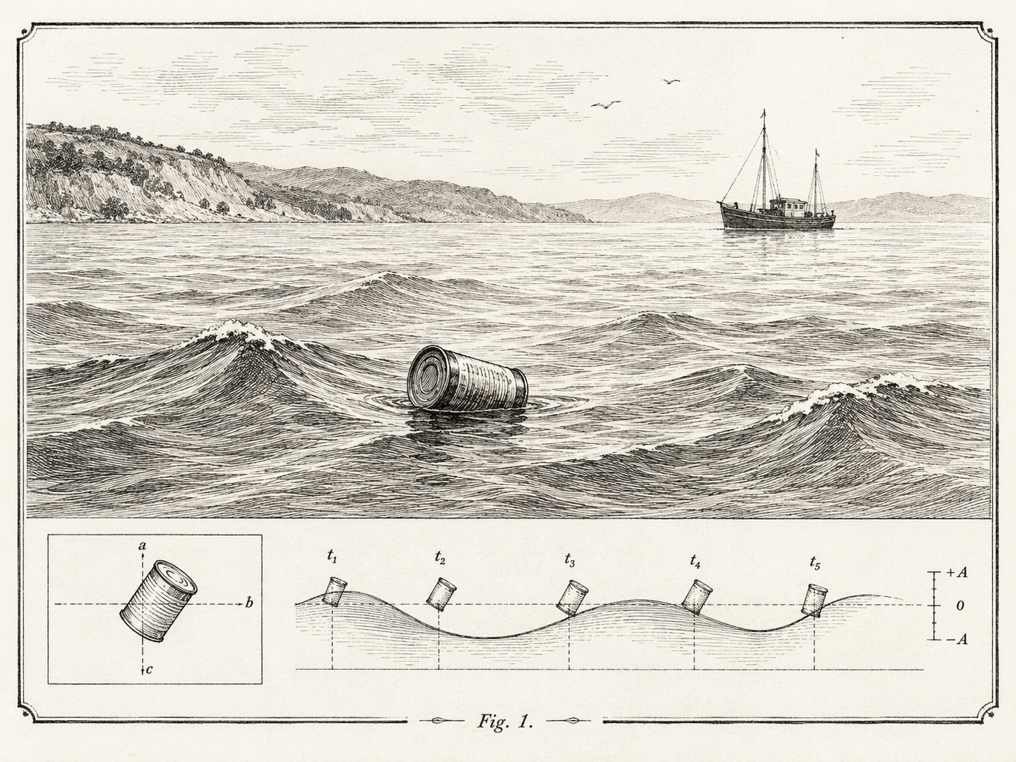
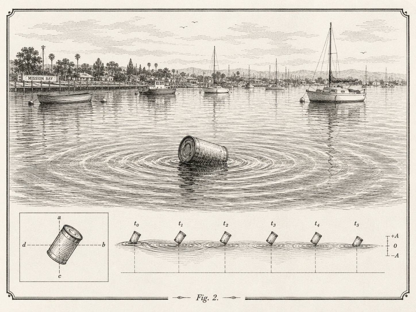
I gave ChatGPT the text of this post and asked it to generate an accompanying image. The results were both wrong and interesting, so I decided to keep them. The left panel depicts waves, but not the kind of waves discussed in the paper. The model imagined something closer to open-water swells, misunderstood the appearance of San Diego’s Mission Bay, chose the wrong type of boat in the background, and invented an implausible horizon and surrounding landscape. I then explained these problems and asked it to try again. The second image is somewhat closer, but still no cigar. Together, the images reveal how little physical grounding current generative models possess. Despite having been trained on millions of images and vast amounts of text, the model failed to infer that the story concerned an empty soda or beer can. More importantly, it appears not to understand the physics of a floating object bobbing on a water surface: the orientation and immersion of the can are inconsistent with the surrounding wave geometry. I kept both images because their failures are instructive. They offer a small visual demonstration of the distance that still separates statistical familiarity with descriptions and images from the structured understanding us humans bring to objects, environments, and the physical world.
I began imagining the can as a kind of local read–write element embedded in a much larger dynamical medium. Perhaps one could define a moving boundary around it—not a rigid box, because the boundary would have to deform and move with the water, but something more like a loose enclosure made of ropes. The purpose of this imagined boundary would be to separate the local interaction from the global field without isolating the two.
Inside that boundary, the can would interact with the wave at one location. But the bay was vastly larger, and every local disturbance contributed to a field that propagated globally. The same wave was therefore both local and nonlocal: sampled at the position of the can, yet distributed across the entire medium.
That was the beginning of my thinking about physical computation, local readout, distributed memory, and closure.
At the same time, I have also been working on cortical traveling waves—developing methods for wave decomposition and thinking about generative models of traveling-wave dynamics using modern machine-learning ideas, including Koopman-based representations (unpubplished works). Those projects have taken their own circuitous path through the current disorder of the American scientific funding system. The proposal is still waiting for review. NSF, please do your job. At this point, I may also need a patron saint.
But scientifically, the connection was natural. Cortical waves are distributed physical processes. Local neuronal populations both respond to those waves and contribute to their propagation. Information is neither stored at a single point nor located entirely in the global field. It emerges through the interaction between local dynamics, distributed state, memory, and recurrence.
The question from Mission Bay therefore returned in a more serious form:
When does a physical wave field merely evolve, and when does a system coupled to that field compute?
An important step came when I read the elegant experiment by Perrard, Fort, and Couder, “Wave-Based Turing Machine: Time Reversal and Information Erasing.”
In their system, a droplet bounces on a vertically oscillating liquid bath and generates a persistent wave field. The droplet is then guided by the local slope of the very field created by its previous impacts. Its trajectory is written into the wave, stored for a finite time, and subsequently read through the droplet–wave interaction. Under an imposed phase shift, the droplet can retrace part of its previous trajectory while progressively erasing the stored wave field.
It is a beautiful physical realization of writing, storage, reading, feedback, and erasure.
But it also sharpened the conceptual difficulty. Are these ingredients sufficient for computation? Does physical memory automatically imply computation? Is a system computing because an observer can interpret its state evolution computationally, or must the computational organization be realized within the physics of the system itself?
It took several years to determine how I wanted to approach these questions.
Eventually, together with my mathematician friend and collaborator Gianluca Caterina, I developed a category-theoretic framework for physical computation. That work became “Physical computing: a category theoretic perspective on physical computation and system compositionality.”. (Also see “the companion post to that work”).
The categorical framework gave us a formal language for relating physical processes to abstract computational processes while preserving their structure. It also allowed us to think systematically about composition, multiple realizability, scale, and the relationship between local physical operations and higher-level abstractions.
Once that foundation was in place, I could return to the original wave problem.
The remaining step was to ask what distinguishes a physical system with memory from a physically closed computational system. A wave reservoir may contain a detailed record of its past. A localized probe may read from it and perturb it. But autonomous computation requires something more: the system’s own physical readout must participate in selecting what operation occurs next.
This is where the connection to reservoir computing becomes natural. A reservoir contains a high-dimensional dynamical state shaped by its input history. A readout extracts task-relevant structure from that state. But in most reservoir-computing systems, the readout remains external: it observes the reservoir without becoming part of the physical causal loop that determines the reservoir’s next operation.
The paper develops a closure criterion for when that readout becomes internalized—when memory, readout, control, and subsequent physical evolution form a closed computational organization.
This also connects with my broader work on opening the black box of recurrent systems and understanding how their internal dynamics support computation—for example, in this recent work on reservoir computing and spatiotemporal chaos. (Also see “the companion post to that work”).
I wrote this companion piece because the final paper sits at the intersection of several fields. Physicists may recognize the wave dynamics but not the category theory. AI researchers may recognize reservoirs and recurrent computation but not the physical-computational problem. Neuroscientists may recognize traveling waves and distributed recurrence but not the formal machinery used to connect them.
The purpose here is to make the union more accessible: to explain how a can bobbing in Mission Bay led, through wave memory, cortical dynamics, category theory, and reservoir computing, to a criterion for autonomous physical computation.
Enjoy—and stay tuned. There is more coming on this front.
And I am still accepting applications for a patron saint.
As for the beautiful woman in the hotel room: it probably would not have worked in the long run. The conversation was pleasant, but my attention had already been captured by a floating can and the computational ontology of waves.
A droplet that walks backward through its own memory
There is an experiment in fluid dynamics that should unsettle anyone who thinks they know where the boundary between “physics” and “computation” lies.
Place a millimetric droplet on a bath of silicone oil vibrated just below the Faraday instability threshold. The droplet bounces indefinitely, never coalescing, and at each bounce it excites a standing surface wave. Because the bath is driven close to threshold, these waves decay slowly — the surface becomes a fading record of everywhere the droplet has recently been. The droplet, in turn, is propelled by the local slope of this self-generated field. It writes to the bath, and the bath guides it. The result — the “walker” of Couder, Fort, and colleagues — is neither a passive particle nor a prescribed wave packet, but a recurrent wave–particle entity guided by its own history.
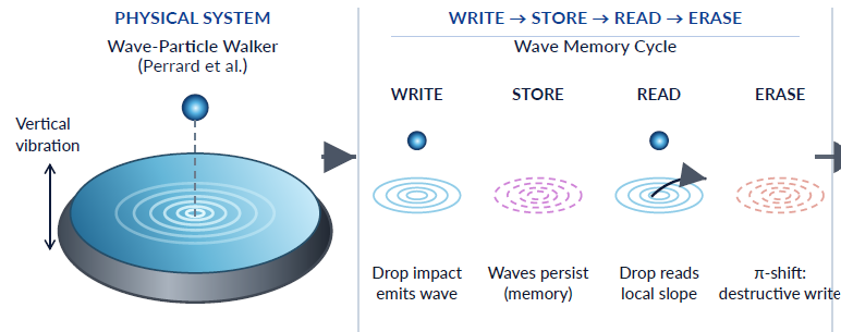
Then comes the striking part. Perrard, Fort, and Couder showed that if you impose a controlled $\pi$-phase shift between the droplet’s bounce and the preexisting wave field, the effective wave-induced kick reverses sign. In confined chaotic regimes, the droplet doesn’t merely reverse velocity — it transiently retraces its own complex trajectory, reading its stored wave memory backward. And as it backtracks, the freshly emitted waves are written in antiphase with the old field, destructively interfering with it. The walker reads its memory backward while physically erasing it.
Writing. Storage. Reading. Feedback. Reversal. Erasure. The vocabulary of a Turing machine, embodied in oil and vibration. Perrard and colleagues framed the experiment in exactly those terms — a “wave-memory Turing machine.”
The question my paper asks is the one this framing forces on us: does a physical system that writes, stores, reads, and erases information thereby compute? And if not, what exactly is missing — not metaphorically, but as a matter of state spaces, dynamics, and physically checkable conditions?
The answer I develop is a hierarchy with a sharp final rung:
\[\text{physical memory} \;\rightarrow\; \text{transition-preserving physical computation} \;\rightarrow\; \text{closed autonomous physical computation}.\]The walker occupies the first rung magnificently and gestures at the second. It does not reach the third — and the reason it doesn’t turns out to be a design principle, one that applies far beyond hydrodynamics: to neuromorphic hardware, physical reservoir computers, and arguably to how we should think about computation in nervous systems.
Let me build this up from the physics.
The walker as a stroboscopic reservoir
The first move in the paper is to strip the walker down to the minimal dynamical structure needed to talk about memory, readout, erasure, and computation — without losing what makes it physical.
The system has a natural clock: the Faraday period $T_F$. Stroboscoping at impact times $t_n = nT_F$, the physical state at bounce $n$ is
\[x_n = (\mathbf{r}_n, \mathbf{v}_n, \sigma_n, H_n) \in X,\]where $\mathbf{r}_n$ and $\mathbf{v}_n$ are the droplet’s horizontal position and velocity, $\sigma_n \in {+1,-1}$ is its bouncing phase relative to a fixed Faraday phase, and $H_n$ is the surface-wave field over the bath — the memory. The field lives in a function space $\mathcal{H}$ (something like $H^1(\Omega)$, since the droplet responds to slope).
| Each bounce writes a localized Faraday source into the bath — in the Bessel approximation, $\psi_{\mathbf{r}}(\rho) = h_0 J_0(k_F | \rho - \mathbf{r} | )$ — and the field updates as |
where $M_e = \tau / T_F$ is the dimensionless memory parameter: the wave decay time measured in Faraday periods. Iterating, the field is an exponentially weighted trace of the droplet’s own past:
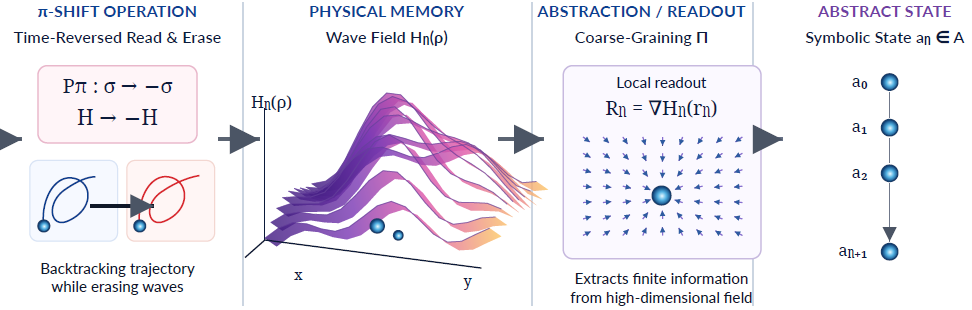
\[H_n = \sum_{q=1}^{n} \lambda^{q-1} \, \sigma_{n-q} \, \psi_{\mathbf{r}_{n-q}}.\]This is the storage half of the loop. The reading half is strikingly local: the droplet does not perceive the global field. It samples only the slope at its own impact point,
\[\mathbf{g}_n = \nabla H_n(\mathbf{r}_n),\]and receives a horizontal kick $-\kappa\,\sigma_n \nabla H_n(\mathbf{r}_n)$ at the next bounce, alongside persistence, confinement, and noise:
\[\mathbf{v}_{n+1} = a\,\mathbf{v}_n - \kappa\,\sigma_n \nabla H_n(\mathbf{r}_n) - \chi \nabla V(\mathbf{r}_n) + \boldsymbol{\xi}_n, \qquad \mathbf{r}_{n+1} = \mathbf{r}_n + T_F \mathbf{v}_{n+1}.\]The factor $\sigma_n$ deserves a word, because it is doing quiet but essential work. The droplet samples the field at its own bouncing phase, so the wave-mediated force is $\mathbf{F}^{\mathrm{wave}}_n = -C\,\sigma_n \nabla H_n(\mathbf{r}_n)$. In the phase-locked regime this factor is inert — $\sigma_n$ squares against the phases carried by $H_n$ and the standard guidance is recovered. Its role is to make the phase a live variable in the force law, which is what allows a phase intervention to act on the dynamics at all. Without it, flipping $\sigma$ would change nothing about the kick, and the erasure story below would not follow from the equations.
Together these define a stroboscopic map $x_{n+1} = F(x_n)$ — a discrete-time reduction of the Oza–Rosales–Bush trajectory equation that retains the memory kernel and the local-slope coupling while suppressing within-bounce hydrodynamics.
Written this way, the walker is a physical reservoir system. The extended field $H_n$ is a high-dimensional memory reservoir; the droplet is simultaneously a localized probe and a localized actuator; and the readout $\nabla H_n(\mathbf{r}_n)$ feeds back into future motion and future writing. This identification is not decorative — it is what lets the closure criterion, derived on the walker, transfer to reservoir computing at the end.
Memory and erasure, made quantitative
“Wave memory” here is not a metaphor and not an observer’s reconstruction. Two facts make it physical.
Finite horizon. Truncating the trace to the last $L$ impacts incurs an error bounded by
\[\|H_n - H_n^{(L)}\|_{\mathcal{H}} \leq \Psi_0 \frac{\lambda^L}{1-\lambda},\]so at fixed field resolution the effective memory horizon scales as $L_{\mathrm{eff}} \sim M_e$. The memory parameter is not a knob on a model; it is a physically tunable memory depth.
Causal readability. The stored field enters the equation of motion through $\nabla H_n(\mathbf{r}_n)$. The memory affects the future. This is what separates a dynamical memory from a mere record that only an external observer could decode.
Erasure gets an equally physical definition. The $\pi$-shift is an operation on state,
\[P_\pi : (\mathbf{r}, \mathbf{v}, \sigma, H) \mapsto (\mathbf{r}, \mathbf{v}, -\sigma, H),\]which does not touch the stored field directly. Instead, all subsequent writing happens in antiphase. Decomposing the field $m$ bounces after the shift into the decayed old memory $H_{\mathrm{old}}^{(m)} = \lambda^m H_{n_\pi}$ and the newly written antiphase contribution $H_{\mathrm{new}}^{(m)}$, erasure is the condition that new writing reduces the field energy beyond passive decay:
\[\|H_{\mathrm{old}}^{(m)} + H_{\mathrm{new}}^{(m)}\|^2 < \|H_{\mathrm{old}}^{(m)}\|^2,\]i.e. genuine destructive interference between the new sources and the stored trace. Because the coupling carries $\sigma_n$, the same phase flip reverses the effective kick exerted by the preexisting field, $-C\sigma_+\nabla H \mapsto +C\sigma_+\nabla H$, producing finite-time backtracking over a horizon of order $M_e/2$. Note what this does not say: the droplet’s interaction with the new, antiphase sources it is now laying down is perfectly normal. Only its relation to the stored past is inverted. Not global time-reversal invariance — memory-mediated, finite-horizon reversal, with the memory consumed in the act.
So the walker has, demonstrably and quantitatively: writing, finite-time storage, local reading, closed analog feedback, finite-time reversal, and physically real erasure. These are genuine information-processing primitives. And here is the pivot of the whole paper: they are still not sufficient for computation.
What computation demands: coarse-grained transition preservation
Physical memory is not yet computation. A magnetized material “remembers” its field history; a deformed solid retains a record of its loading; a memristive element carries a trace of past current. Rich, dynamically consequential memory is everywhere in physics. Something more is needed, and the paper’s first criterion pins it down.
Let $F : X \to X$ be the physical dynamics and $G : A \to A$ an abstract transition rule on an abstract state space $A$ — the “program level.” A coarse-graining $\Pi : X \to A$ implements $G$ on a domain $U \subseteq X$ when the diagram commutes:
\[\Pi \circ F = G \circ \Pi \qquad \text{on } U.\]Physically evolve then abstract, or abstract then formally step — you land in the same place. The abstraction is not a label painted on after the fact; the dynamics respects it.
Two features of this condition do the philosophical heavy lifting.
First, $\Pi$ is many-to-one. It induces an equivalence $x \sim_\Pi x’ \iff \Pi(x) = \Pi(x’)$, and the physical dynamics descends to a well-defined abstract rule on the quotient only if
\[\Pi(x) = \Pi(x') \;\Longrightarrow\; \Pi(F(x)) = \Pi(F(x')).\]When this holds, the abstract map $G$ exists and is unique (this is a proposition in the paper). Abstract states are not microstates — they are equivalence classes, macrostates, basins. This replaces the overly strong demand of one-to-one physical–symbol identity, which no real computer satisfies anyway.
Second, and pulling in the opposite direction, the commutation requirement is exactly what blocks the overly weak view — Putnam- and Chalmers-style arguments that any physical system “computes” anything you can map onto it. An arbitrary labeling won’t commute with the dynamics. The mapping must be preserved by the physics, step after step. That single equation is the wall between computation and relabeling.
This criterion has a lineage worth naming. Abstraction/representation (AR) theory framed computation as a commuting relation between physical dynamics and an evolving representation, but placed no restriction on the representation — leaving it exposed to the simple-mapping objection. The mechanistic account demands robust, functionally individuated structure but stays descriptive, without a concrete tie to dynamics. The categorical framework Gianluca Caterina and I developed previously casts the relation as a functor between a category of physical processes and one of abstract processes. This paper instantiates that framework on an explicit physical substrate and, as we’ll see, pushes it one step further — because putting it on a concrete substrate exposes a question the abstract formulation never had to confront.
Robust symbolization: computation must survive noise
Exact commutation is an idealization. Real systems are noisy and finite-resolution, so the paper’s second criterion replaces exact symbols with separated basins.
For a finite abstract alphabet $A = {a_1, \ldots, a_K}$, each symbol $a_i$ is realized by a physical region $B_i \subset X$, and robustness requires the basins to be distinguishable at the physical uncertainty scale $\varepsilon_X$:
\[\operatorname{dist}(B_i, B_j) > 2\varepsilon_X, \qquad i \neq j,\]with transitions that remain reliable under stochastic dynamics:
\[K(x, B_{g(i)}) \geq 1 - \delta \qquad \text{for } x \in N_{\varepsilon_X}(B_i),\]where $K$ is the transition kernel. A symbol is a basin you can’t accidentally fall out of; a transition is a basin-to-basin map that holds with probability at least $1-\delta$.
This framing makes the failure modes of physical computation just as precise as the success condition: aliasing (basins that overlap at resolution $\varepsilon_X$), representative dependence (two microstates in one basin evolving into different basins — the commutation condition failing), noise-induced basin crossing, and transition deformation.
One failure mode is specific to wave reservoirs and worth singling out: memory decay. Two wave-memory states separated by $D_0$ converge under passive decay as $D_m \approx \lambda^m D_0$, becoming physically indistinguishable after
\[m \gtrsim M_e \log\!\left(\frac{D_0}{2\varepsilon_H}\right)\]bounces. The memory parameter doesn’t just set how long the walker remembers its path — it bounds the reliable lifetime of any memory-dependent symbolic distinction the system could support. A fading reservoir imposes a hard expiration date on its own alphabet. Any wave-based computing architecture must either operate within this horizon or actively refresh its symbols.
The closure criterion: who selects the next operation?
Now the central step — the paper’s core contribution.
Suppose a system passes everything so far: it has memory, separated basins, robust transition preservation. It can still fail to be a computer in an important sense, because everything above can hold while an external agent supplies the operations. If $\mathcal{O}$ is a set of physically realizable operations $F_o : X \to X$ and an experimenter schedules the sequence $o_0, o_1, \ldots$, the evolution
\[x_{n+1} = F_{o_n}(x_n)\]may implement perfectly valid abstract transitions — but the selection of what happens next lives outside the system. This is exactly the walker’s situation: the $\pi$-shift, the one operation that triggers reversal and erasure, is imposed by the experimenter’s function generator.
Closure is the condition that operation selection be internal. Decompose the state space as
\[X = X_R \times X_Y \times X_Z,\]where $X_R$ is the reservoir/memory subsystem and $X_Y$ is a physical readout-control subsystem. Let $y_n = p_Y(x_n)$ be the readout state and $C : X_Y \to \mathcal{O}$ a physical operation-selection map. The closed-loop evolution is
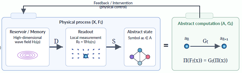
\[\boxed{\,x_{n+1} = F_{C(y_n)}(x_n) = F_{C(p_Y(x_n))}(x_n)\,}\]The readout is not merely observed — it is coupled back into the dynamics, choosing what the system does next. Writing $\Phi(x) = F_{C(p_Y(x))}(x)$ for the resulting autonomous map, closed physical computation is the compatibility of this loop with the abstraction: $\Pi(\Phi(x)) = G(\Pi(x))$, or with operation-dependent abstract rules, $\Pi(\Phi(x)) = G_{\Theta(C(p_Y(x)))}(\Pi(x))$.
Two clarifications sharpen what closure is and is not.
Closure is not feedback. The walker already has a beautiful closed analog loop: $H_n \to \nabla H_n(\mathbf{r}n) \to \mathbf{v}{n+1} \to H_{n+1}$. Feedback is ubiquitous — a driven pendulum has it, a chemical oscillator has it. Closure requires something structurally stronger: a readout state that selects among distinct operations — normal propagation vs. phase flip vs. confinement change — not a continuous variable that merely modulates one flow. (The supplement makes this precise with nondegeneracy conditions separating genuine operation selection from continuous feedback.)
Closure is not computational power. This is a boundary the paper draws deliberately. A two-state controller that flips $o_{\mathrm{normal}} \leftrightarrow o_\pi$ every step is closed, transition-preserving, and autonomous — and computes nothing of interest. Closure marks the line between externally driven and autonomous physical computation, not between weak and powerful computation. Richness — a sufficient alphabet, programmable transitions, composable operations — is a separate, further requirement.
The categorical lift: where does the morphism come from?
Why bring category theory into a fluid-dynamics paper? Not as ornament. The dynamical-systems statement of closure leaves three things implicit that the categorical formulation makes structural.
In the framework from my earlier work with Caterina, physical processes form a category $\mathbf{PhysProc}$ (objects: physical regions; morphisms: physically realizable processes), abstract transitions form $\mathbf{AbsProc}$, and computation is a functorial relation between them. The coarse-graining descends to a quotient functor
\[Q_\Pi : \mathbf{PhysProc}_\Pi \to \mathbf{AbsProc}, \qquad Q_\Pi(F) = G \iff \Pi \circ F = G \circ \Pi,\]defined on the subcategory of processes that respect $\Pi$-equivalence. Abstraction and concretization, $\alpha(U) = \Pi(U)$ and $\gamma(S) = \Pi^{-1}(S)$, form a Galois-style pair,
\[\alpha(U) \subseteq S \iff U \subseteq \gamma(S),\]and transition preservation becomes basin containment: $F(B_a) \subseteq B_{G(a)}$. In noisy systems, strict functoriality relaxes to an approximate quotient functor $Q_\Pi(F) \approx_{\varepsilon,\delta} G$, with $\varepsilon$ tracking resolution and $\delta$ bounding transition failure. This is the formal home of the intuition that computation is about processes respecting a quotient — many microstates per symbol, adjunction rather than bijection, the middle path between physical–symbol identity and arbitrary mapping.
But instantiating this machinery on the walker’s explicit state space exposed a question the functorial picture never had to confront: at each step, what chooses the morphism? In AR theory and in the functorial formulation alike, the operation is handed to the diagram from outside. Closure is the condition that the system choose it. Categorically, the closed-loop morphism is
\[\Phi = \mathrm{Act} \circ \langle C \circ p_Y, \;\mathrm{id}_X \rangle, \qquad \mathrm{Act}(o, x) = F_o(x).\]Read this composite carefully. The pairing $\langle C \circ p_Y, \mathrm{id}_X \rangle$ sends $x \mapsto (C(p_Y(x)), x)$: the system’s own state produces both the operation and the operand. The external index $o \in \mathcal{O}$ has been eliminated from the diagram — replaced by a value of the system’s own readout. Coalgebraically, $\Phi$ equips $X$ with the structure of a transition system whose next-step map factors through an internal observation rather than an external driver. Autonomy stops being an interpretive gloss and becomes a structural property of how the process is generated.
The verdict on the walker
With the hierarchy in hand, the classification is precise, and it is neither a debunking nor an endorsement of the “wave Turing machine” framing.
The walker has: physical memory ($H_n$ as an exponentially weighted trace), physical writing ($H_{n+1} = \lambda H_n + \sigma_n \psi_{\mathbf{r}_n}$), finite-time storage (horizon $\sim M_e$), physical local reading ($\nabla H_n(\mathbf{r}_n)$ entering the equation of motion), closed analog feedback, physically real erasure (the destructive-interference inequality), and finite-time memory-mediated reversal.
The walker lacks, as experimentally realized: a demonstrated symbolic transition system $(A, \Pi, G)$ with $\Pi \circ F = G \circ \Pi$; separated basins with reliable transitions serving as an alphabet; and — decisively — closure. The $\pi$-shift is imposed externally. There is no internal readout state $y_n$ with $C(y_n) = P_\pi$.
\[\boxed{\text{wave-memory physical machine with Turing-like primitives}} \quad \text{but not} \quad \boxed{\text{closed autonomous Turing machine}}\]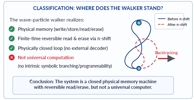
The point of this classification is that the missing layer is not mysterious. It is a specific, buildable subsystem — and that turns the criterion into a research program.
Closing the loop: from criterion to blueprint
If closure is what’s missing, add it. The constructive section of the paper proposes physical architectures of the form
\[y_{n+1} = \mathcal{R}(y_n, H_n, z_n), \qquad o_n = C(y_n), \qquad (H_{n+1}, z_{n+1}) = F_{o_n}(H_n, z_n),\]where $z_n = (\mathbf{r}_n, \mathbf{v}_n, \sigma_n)$ and the readout $y$ is a physical degree of freedom, not a camera feed into a laptop. Candidate implementations:
A multistable readout. A coordinate $y$ in a double-well potential $U_Y(y;q) = \frac{\alpha}{4}y^4 - \frac{\beta}{2}y^2 - \gamma q y$, tilted by a scalar $q_n$ extracted from the wave state (a projected slope, or an integrated field $\int_\Omega \chi(\rho) H_n(\rho)\,d\rho$). The two wells $Y_\pm$ are the readout basins; $C(Y_+) = o_\pi$, $C(Y_-) = o_{\mathrm{normal}}$. The phase flip becomes wave-triggered.
A thresholded, hysteretic wave detector. The cleanest decisive experiment — an autonomous eraser. Let the readout track the normalized wave energy $E_W[n] = |H_n|{L^2}^2 / |\psi{\mathbf{0}}|_{L^2}^2$ through a hysteretic threshold:
\[y_{n+1} = \begin{cases} 1, & E_W[n] > \Theta_E,\\[2pt] 0, & E_W[n] < \Theta_E - \Delta,\\[2pt] y_n, & \text{otherwise}, \end{cases} \qquad C(0) = o_{\mathrm{normal}}, \quad C(1) = o_\pi.\]The loop $H_n \to E_W[n] \to y_n \to o_\pi \to \text{erasure}$ means the system erases its own memory when its own field crosses a physical threshold. The critical experimental comparison is three-way: an external phase schedule (the current experiment), observer-side readout without feedback, and physical readout with feedback. Only the third satisfies closure — and hysteresis is essential, because it is what makes the readout a genuine two-basin state rather than a relabeled continuous variable.
Boundary-controlled reservoirs and coupled walkers. The readout can also select bath parameters — memory depth $\lambda(y_n)$, forcing phase, confinement geometry — making the wave update itself state-dependent. Or a second walker in the same bath, interacting through the superposed field $H_{n+1} = \lambda H_n + \sigma_n^A \psi_{\mathbf{r}n^A} + \sigma_n^B \psi{\mathbf{r}_n^B}$, can serve as a finite-state controller embedded in the very substrate it controls.
The design principle, boxed in the paper:
\[\boxed{\;\text{wave memory} \;+\; \text{intrinsic readout basins} \;+\; \text{state-dependent operation selection} \;=\; \text{closed physical computation}\;}\]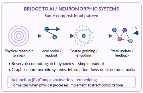
What this means for physics
A falsifiable criterion where there was a metaphor. “This system computes” has too often been an interpretive flourish attached to interesting dynamics. The framework replaces it with conditions you can check in the lab: exhibit the basins, measure their separation against the noise scale $\varepsilon_X$, verify transition reliability $1-\delta$, and identify — or fail to identify — the internal readout-to-operation coupling. The three-way autonomous-eraser comparison is a concrete experiment with a binary outcome. Computation claims about physical systems become experimental claims.
A hierarchy that organizes a zoo. Memristive materials, magnetic hysteresis, shape memory, vortex records, wave fields: physics is full of systems with memory, and the literature is full of debates about which of them “compute.” The three-rung ladder — memory, transition preservation, closure — gives these debates a shared coordinate system. Most memory materials sit on rung one. Externally clocked, externally read devices can reach rung two. Rung three is rare and architecturally specific, and that is precisely what makes it a meaningful target.
Memory depth as a computational resource with hard bounds. The result $m \gtrsim M_e \log(D_0 / 2\varepsilon_H)$ ties an abstract computational property — how long a symbolic distinction can persist — to a measurable physical parameter. For any fading-memory substrate (near-threshold waves, decaying spin textures, leaky photonic cavities), this bound tells you the symbol lifetime your physics can support before refresh is mandatory. It is the kind of exchange rate between physical and computational quantities that a physics of computation should be producing.
A disciplined answer to pancomputationalism. Does a rock compute its trajectory? Does the Solar System compute Newton’s laws? The framework’s answer is a firm no, not in the relevant sense — but for a physicist’s reason, not a philosopher’s. What the rock lacks is not complexity or observers; it lacks a physically organized coarse-graining whose transitions the dynamics preserves robustly, and any readout-control organization at all. The contrast case is the billiard-ball computer: a generic moving ball is not a logic gate, but a ball in a constrained collision architecture is, because the constraints organize the physics to preserve an abstract transition structure. Computation is a property of physical organization, not of physical evolution per se — a statement that rejects arbitrary mappings without denying that unconventional, analog, quantum, or wave-based substrates can genuinely compute.
And a caveat physics should respect. The criterion is deliberately minimal. It says nothing about computational power, efficiency, thermodynamic cost, or universality — a closed system can be trivially closed. Universality would require a robust alphabet, programmable transitions, addressable memory, scalable composition. The paper stops at the prior question, because the prior question — is the system autonomous or externally driven? — had no sharp answer before.
What this means for neuroscience (and why NeuroAI needs it)
Neuroscientists say “this circuit computes” constantly, and almost never say what would make it false. The word usually means one of three very different things — that the activity carries information about a stimulus, that it transforms inputs into outputs, or that it implements an algorithm — and the slide between them is so frictionless that it rarely gets noticed. The framework above is, among other things, a way to stop sliding. Let me translate it out of the oil bath.
The three rungs, in neural terms
Rung one: memory. A circuit’s current state carries information about its past. This is nearly free. Synaptic traces, short-term facilitation, slow adaptation currents, persistent activity, the after-effects of a traveling wave — all of it is memory in the sense used here. A dissipative system with a fading trace of its own history is not rare; it is the default condition of nervous tissue. Finding memory in a circuit tells you almost nothing about whether it computes.
Rung two: transition preservation. Now there is a coarse-graining $\Pi$ from neural states to some abstract description — task states, decision variables, latent factors, phases of a sequence — and the neural dynamics respect it: evolving the circuit and then abstracting gives the same answer as abstracting and then applying the abstract rule, $\Pi \circ F = G \circ \Pi$. This is a real constraint, and it is what most careful computational neuroscience is actually claiming when it says a circuit “implements” something. The robustness layer matters here too: the abstract states must be separated basins in the neural state space, distinguishable at the scale of the circuit’s own noise, with transitions that hold reliably. A latent variable you can extract from population activity is not automatically a symbol the circuit itself can act on.
Rung three: closure. The circuit’s own readout state selects what the circuit does next. Not “influences” — selects, from among distinct operations.
That third rung is where the interesting claim lives, and where neuroscience has been unwittingly ambiguous.
The decoding fallacy, named
Here is the uncomfortable observation. The single most common methodology in systems neuroscience is: record a population, train a decoder, report that the decoder recovers some variable with high accuracy, and conclude that the region encodes, represents, or computes that variable.
Look at what that experiment actually establishes, in the framework’s terms. It establishes that an observer-side readout exists — that you, with a GLM or an SVM or a linear projection, can recover the variable. It establishes precisely nothing about whether the brain reads it. The decoder is your classifier, running on your laptop, downstream of nothing.
Recall the three-way experimental comparison the paper proposes for the walker:
- an external operation schedule,
- observer-side readout without feedback,
- physical readout with feedback.
Only the third satisfies closure. And condition 2 — observer-side readout with no causal path back into the dynamics — is a description of a decoding study. It is the control condition. Neuroscience has industrialized the control condition and, in a great deal of its rhetoric, reported it as the result.
This is not a claim that decoding is bad science; it is indispensable, and it establishes that the information is there. It is a claim about what the inference licenses. Decodability is a statement about the mutual information between neural activity and a variable. Computation, in the sense that would justify the word, is a statement about causal architecture: whether some physical state of the circuit is coupled back into the circuit’s own subsequent operations. Those are different claims, and only the second one is about the brain rather than about the experimenter.
Notice this is the same error, structurally, that the walker experiment makes — and the walker’s version is more honest, because there the external agent (the function generator imposing the $\pi$-shift) is visible on the bench. In a decoding study the external agent is the analysis pipeline, and it is easy to forget it is there at all.
What closure would actually require of a circuit
So what would it take to earn the word? You would need to identify, physically:
- A readout variable inside the circuit. Not a latent factor in your dimensionality reduction — a physical degree of freedom. Downstream spiking in a target population. A dendritic nonlinearity crossing threshold. A neuromodulatory state. A bistable attractor in a gating circuit. It has to be made of neurons, not of PCA.
-
Distinct operations for it to select among. This is the condition people skip. Closure requires more than that the readout modulates an ongoing flow — that is just feedback, and feedback is everywhere (recurrent excitation, adaptation, gain control, every loop in the brain has it). Closure requires that the readout state select among qualitatively different things the circuit can do: gate this pathway or that one, write to memory or erase it, switch dynamical regime, route to a different downstream target. Formally, the operation-selection map must be nontrivial, $ \mathrm{Im}(C) \geq 2$. A circuit whose recurrent activity smoothly tunes its own gain is a beautiful feedback system and is not, on that basis alone, closed. - A causal path from the readout back into the dynamics. Perturb the readout state; the subsequent operation changes. That is an intervention, not an observation — and it is why optogenetics, not electrophysiology, is the natural instrument for testing closure.
Written this way, the criterion turns into an experimental program: identify the candidate readout, show it occupies separated basins, show that basin membership predicts which operation the circuit performs next, and show that forcing the basin forces the operation.
And here is the part worth sitting with: nervous systems very likely are closed, and that is a substantive structural fact, not a truism. Neural activity does not merely represent states for an external observer — it acts on downstream circuits, gates future processing, opens and closes routing pathways, and changes the physical conditions under which later activity unfolds. At the cellular scale the point is even sharper: ion channels function simultaneously as the readout and the control variable, which is closure in miniature. The brain is not a reservoir waiting to be decoded. It is a system that reads itself and acts on what it reads. That is precisely the property that almost every engineered “physical computer” lacks — and it may be the most underrated thing about biological computation.
Traveling waves as the test case
The same discipline applies to what is currently one of the most enthusiastic corners of the field. Cortical traveling waves propagate, modulate excitability, organize spike timing, and structure spatiotemporal activity. Do they compute?
Under this criterion, the question stops being about appearance and becomes about architecture. A wave becomes computationally relevant when you can identify the physical variables it transforms, the coarse-grained states it stabilizes or routes, and the downstream readout/control pathways through which it changes later neural dynamics. Not whether the activity pattern visually resembles a wave. Whether the readouts form robust, transition-preserving, closed loops.
I want to be careful about the analogy, because it is easy to abuse. The claim is emphatically not that cortex is a hydrodynamic walker. It is structural and limited: both systems contain distributed wave-like activity, local readout, and recurrent physical coupling. In the walker, the readout is the droplet sampling $\nabla H(\mathbf{r})$. In cortex, the readout might be downstream spiking, synaptic integration, dendritic nonlinearities, local thresholds, or long-range recurrent coupling. What transfers is the question, not the substrate.
The research program this suggests is concrete: do wave variables define robust basins or phase states? Do those states predict — or better, control — transitions in downstream populations? Does perturbing wave phase, direction, or speed change the inferred transition map? And is the relevant readout internal to the circuit, or imposed by your decoder? Cortical waves are, in this sense, an unusually clean biological test case for the closure criterion.
Why NeuroAI needs this, specifically
NeuroAI is a field built on an analogy between two systems whose computational status is asserted far more often than it is defined. That is a precarious foundation, and it produces a recurring pathology: a property is found in a trained network, the corresponding property is found in cortex, and the resemblance is reported as convergence — without either side having said what would make the claim false.
The framework offers a shared coordinate system, and it cuts in both directions.
Toward the models: a deep network’s hidden layer that a linear probe can decode is at rung two at best, and the probe is your probe. The network’s own subsequent computation typically does not depend on the probed variable at all. Meanwhile a large model in a standard serving loop — where an external harness decides when to sample, when to call a tool, when to stop — is, structurally, externally driven, however agentic its behavior looks. Closure asks a question that no benchmark currently asks: who selects the next operation, the system or the harness?
Toward the brains: the criterion demands that “the cortex computes X” be cashed out as a causal architecture with identifiable readout basins and operation selection, rather than as a decoding accuracy. It makes the claim expensive — which is the point. Claims that cost nothing are worth nothing.
And it makes the comparison honest. If nervous systems are closed and current artificial systems mostly are not, that is not a gap to be papered over with an analogy; it is arguably the structural difference between them, and it deserves to be named rather than dissolved into the shared vocabulary of “information processing.” The two fields have been using one word — computation — for at least three distinct properties, and NeuroAI is the place where that ambiguity does the most damage, because it is where the equivocation gets laundered into a scientific claim.
The closure criterion will not tell you what the brain computes. It will tell you what you have to demonstrate before you are entitled to say it computes anything at all.
What this means for AI and ML
The closure criterion was derived on droplets and oil, but its most immediate audience may be people building learning machines out of physics.
Reservoir computing has been benchmarking the wrong loop — or at least, only half of it. The standard architecture (echo state networks, liquid state machines, and their myriad physical implementations in spintronics, photonics, mechanics, and fluids) is: a high-dimensional dynamical reservoir transforms input history into a rich state, and an external, trained readout — usually a linear layer on a computer — extracts the answer. Reservoirs are evaluated by how well that external readout decodes them. The closure criterion exposes the architecture’s structural incompleteness: the decoded state never touches the physics again. In the paper’s terms, physical reservoir computing as standardly practiced lives on rung two — transition-preserving under external readout — and the walker makes this separation unusually visible, because its reservoir (the wave field) and its probe (the droplet) are right there in front of you while the operation selection sits in a function generator.
I want to be precise about where the incompleteness lies, because the obvious fix is not the right one. In other work, I put the reservoir substrate itself under evolutionary selection — evolving size, connectivity, spectral radius, input scaling, and regularization of reservoirs tasked with predicting Kuramoto–Sivashinsky spatiotemporal chaos — rather than accepting the usual fixed random recurrent matrix. The substrate turns out to be richly structured and far from arbitrary: selection conserves a global spectral envelope while directionally refining the slow, low-eigenvalue modes that set the reservoir’s memory timescale; macroscopic modularity locks into a narrow band; connection cost is exponentially pruned within that band. Prediction, in other words, imposes legible structural constraints on the recurrent medium — the substrate is a real object of design, not a bag of random dynamics.
And yet: those reservoirs are still on rung two. Every one of them is decoded by a ridge-regression readout trained offline and living outside the physics. Optimizing the substrate — even beautifully, even in ways that reveal genuine structure–function laws — does not move a system across the closure line, because closure is not a property of the reservoir. It is a property of the loop. This is exactly why the criterion is worth having: it identifies an axis of incompleteness that no amount of substrate engineering can address, and that is invisible to the benchmarks the field currently runs. You can evolve the medium to the edge of what prediction demands and still have built something externally driven.
The stronger benchmark the criterion suggests: can the readout be physically internalized, so that decoded states select subsequent reservoir operations?
\[\text{reservoir} \;\to\; \text{physical readout} \;\to\; \text{operation selection} \;\to\; \text{reservoir}.\]A device that satisfies this is a physically closed reservoir computer: its computational state is not read off after the fact but participates in its own future evolution. For neuromorphic engineering, this is a concrete design axis orthogonal to the usual ones (speed, energy, dimensionality): not “how expressive is your reservoir” but “who selects the next operation — your chip, or your host workstation?” A memristive crossbar whose outputs are digitized, thresholded in software, and fed back through a DAC is externally driven no matter how exotic its materials. The same crossbar with an on-substrate hysteretic element that gates its own update pathway is closed. The criterion gives that difference a name and a test.
Symbols from dynamics, with error bars. The robust-symbolization layer — basins separated by $2\varepsilon_X$, transitions reliable to $1-\delta$, symbol lifetimes bounded by memory decay — is essentially a physical theory of when continuous dynamics supports discrete, reliable information processing. That is a question ML keeps encountering from the other direction: when do RNN hidden states organize into effectively discrete attractors? When do the representations inside a trained network support compositional, symbol-like manipulation? When does an analog accelerator’s noise floor destroy the discrete abstraction its compiler assumes? The framework’s failure taxonomy — aliasing, representative dependence, noise-induced crossing, memory decay, transition deformation — reads like a diagnostic checklist for analog and in-materio ML hardware, and each item comes with an inequality rather than an adjective.
Autonomy as architecture, not vibes. The AI world talks constantly about “agents” and “autonomy,” usually behaviorally. The closure criterion offers a structural definition with teeth: a system is autonomous when its next operation is a function of its own readout state, $o_n = C(p_Y(x_n))$, rather than an externally supplied index. Notice what this does and doesn’t say. A large language model in a standard serving loop — where an external harness decides when to sample, when to call tools, when to stop — is, in this structural sense, externally driven regardless of how agentic its outputs look. A system whose own state gates its subsequent operations (what to update, when to erase, which sub-process to run) is closed regardless of how simple it is. And the paper’s own remark cuts the other way too: closure without richness is trivial — a period-two flip-flop is autonomous and boring. Interesting machine intelligence presumably requires both closure and a rich operation set. Keeping those two requirements separate, rather than blending them into one fuzzy notion of agency, is exactly the kind of conceptual hygiene the formalism enforces.
A bridge to biology that isn’t hand-waving. In recurrent neural systems, readout-like variables act on downstream circuits, gate future processing, and change the physical conditions under which later activity unfolds; at the cellular scale, ion channels function simultaneously as readout and control variables. Nervous systems, in other words, look closed in precisely the structural sense defined here — which suggests the criterion as a common language for comparing engineered reservoirs, unconventional computers, and neural circuits without collapsing them all into the vague claim that they “process information.”
Looping back: physical computing as the real subject
Step back from the droplet, and the paper is an answer to a single old question: what does it take for matter to compute?
The history of that question has oscillated between two failure modes. One extreme makes computation too cheap: if computation is just “a mapping from physical states to abstract states,” then everything computes everything, the rock implements every finite-state machine, and the concept dissolves. The other extreme makes it too expensive: if computation requires exact symbol-by-symbol identity between physical and formal states, then nothing physical computes — not even your laptop, whose “bits” are noisy charge distributions stabilized by basins and error margins.
The resolution developed here threads between them with three moves, each carrying its own mathematics:
- Symbols are basins, not microstates. Physical realization is many-to-one, formalized by a quotient — an adjunction, not a bijection: $\gamma({a}) = B_a$, with $\operatorname{dist}(B_i, B_j) > 2\varepsilon_X$.
- Computation is transition preservation, not labeling. The dynamics must commute with the abstraction, $\Pi \circ F = G \circ \Pi$, robustly under noise. This single requirement dissolves pancomputationalism without special pleading.
- Autonomy is internal morphism selection. The step that had never been formalized: a computer, as opposed to a computed-upon system, selects its own next operation — $\Phi = \mathrm{Act} \circ \langle C \circ p_Y, \mathrm{id}_X \rangle$, the external index eliminated from the diagram.
Memory, preservation, closure. Each rung is physically checkable; each has a categorical expression; and the top rung converts a philosophical dispute into an engineering blueprint.
That last conversion is, to me, the point. The walker experiment showed something genuinely profound: memory can be written into matter by matter, read by matter, and erased by matter, in a continuous wave field with no electronics in sight. The closure criterion neither inflates that result into “hydrodynamic Turing machine” nor deflates it into “just a dynamical system.” It locates it — a wave-memory physical machine with Turing-like primitives, one architectural layer short of autonomy — and then specifies the layer: intrinsic readout basins coupled to operation selection. An autonomous eraser on a vibrating bath would be, to my knowledge, the first system to demonstrably cross the closure line in a continuous physical substrate.
The question is no longer whether wave memory is metaphorically computational. The question is how to build physical architectures in which wave memory, readout basins, and operation selection compose into closed autonomous computation — on an oil bath, in a photonic cavity, on a neuromorphic chip, or in a dish of neurons. The criterion tells you what to build and how to know when you’ve built it.
That is what a physics of computation should look like.
The paper develops each layer in full technical detail, with supplementary sections covering the stroboscopic wave model, erasure energetics, coarse-graining theory, robust symbolization, closure and nondegeneracy conditions, the categorical lift, the walker classification, and constructive extensions. The categorical framework builds on Dehghani & Caterina, J. Phys. Complexity (2024) “Physical computing: a category theoretic perspective on physical computation and system compositionality.”.
Cite this post
@misc{dehghani2026waveMatterCompute,
  author       = {Nima Dehghani},
  title        = {{When Does Matter Compute? Wave Memory, Closure, and the Architecture of
                   Autonomous Physical Computation}},
  year         = {2026},
  howpublished = {\url{https://neurovium.science/posts/pblog-Wave-compute/}},
  note         = {Companion post to: Autonomous Physical Computation: A Categorical
                  Closure Criterion for Physical and Neuromorphic Reservoirs. arXiv
                  (2026). arXiv:2607.23902}
}