What the resolution of a neuron model does to the computation
Companion post to:
How Long Is the Coast of a Neuron? Resolution-Dependent Interaction Order and Computational Capacity
Nima Dehghani
arXiv
DOI: https://doi.org/10.48550/arXiv.2610.19487
@misc{dehghani2026CompRes,
  author       = {Nima Dehghani},
  title        = {{What the resolution of a neuron model does to the computation}},
  year         = {2026},
  howpublished = {\url{https://neurovium.science/posts/pblog-CoastOfNeuron/}},
  note         = {Companion post to: How Long Is the Coast of a Neuron? Resolution-Dependent Interaction Order and Computational Capacity (2026). doi:10.48550/arXiv.2610.19487}
}
How This Paper Began
Chaitin, complexity, information
The paper began, as many things did, in the wreckage of the pandemic.
Everything had been reduced, too abruptly, to rooms, screens, and a strange public simulation of normal life. I spent a great deal of that period thinking about the foundations of physical computation, playing chess against engines that seemed to have acquired a Mikhail Tal temperament, and working on a book about information processing in biological systems. That book is still in preparation. I have been too busy finishing papers and research projects from the last decade to bring it to a proper close, but much of the thinking behind this paper came from that period.
As part of the book, I was speaking with people whose work had shaped how I thought about computation, randomness, biology, and mathematics. One of them was Gregory Chaitin. Yes, that Gregory Chaitin, of algorithmic information theory and Chaitin complexity.
I had been reading Chaitin’s work on metabiology, his attempt to think about evolution as a kind of open-ended software process. Some parts of it caught my attention immediately. In Chaitin’s information-theoretic incompleteness theorem, a formal system has a finite informational scale. If its axioms contain only so many bits, then there are hard limits on what it can prove about the complexity or randomness of objects beyond that scale. A system cannot, from within a fixed budget of axioms, certify arbitrary complexity. There is an informational ceiling built into the formal description itself.
Metabiology pushes that idea into a stylized picture of evolution: digital organisms climbing an unbounded landscape of increasing algorithmic complexity. The model deliberately removes much of the physical world. No metabolism, no finite body, no material cost of memory, no ecological limit on the length of the code. Evolution becomes a mathematical process of open-ended search. That abstraction is precisely what makes it powerful, but it also made me think about what happens when physical scale re-enters the story.
My long Zoom conversations with Chaitin took place in late mid 2021, last of them on May 21. They were among the few Zoom conversations from that period that I actually enjoyed. I hated Zoom with unusual passion. It was not only the inconvenience; it was the flattening. Encounters that should have had space, timing, posture, and peripheral presence were compressed into rectangles. Human beings were projected into two-dimensional tiles, and then we all pretended that the projection was the meeting.
That irritation was probably already part of the idea, although I did not yet know it.
Tyler Hobb’s Fidenza
A little later, while rereading my notes and letting the Chaitin conversation settle, I came across Tyler Hobbs’s Fidenza, released in early June 2021. I was immediately drawn to it, not simply as an artwork but as a computational object. Fidenza was not a single image in the ordinary sense. It was a generative recipe: a rule system with controlled variation, producing individual works at minting. The pieces differed in palette, density, texture, turbulence, collision, and scale. Some were dominated by large, block-like forms; others were dense with small filaments and delicate local structure.
What interested me was not the usual surface description of generative art. It was the coexistence of a hidden rule and a visible scale. A few mathematical choices could make the same canvas look sparse or crowded, massive or filamentary, calm or turbulent. The computer was drawing blindly in one sense, but it was not drawing randomly. The paths were guided by a hidden field.
Here are some beautiful examples of Fidenza that Tyler sent me that I can share on this blog post (Thank you Tyler!):


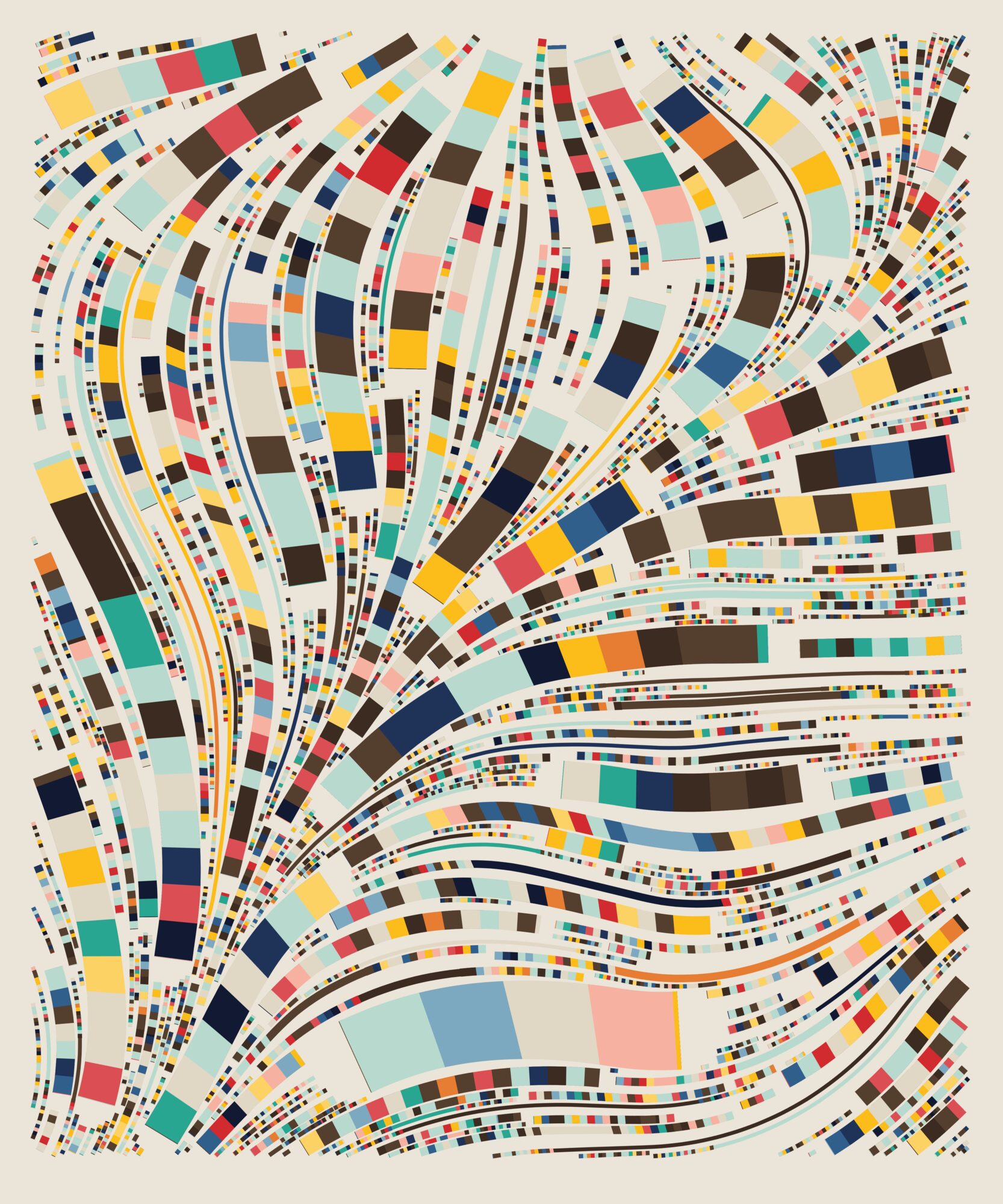
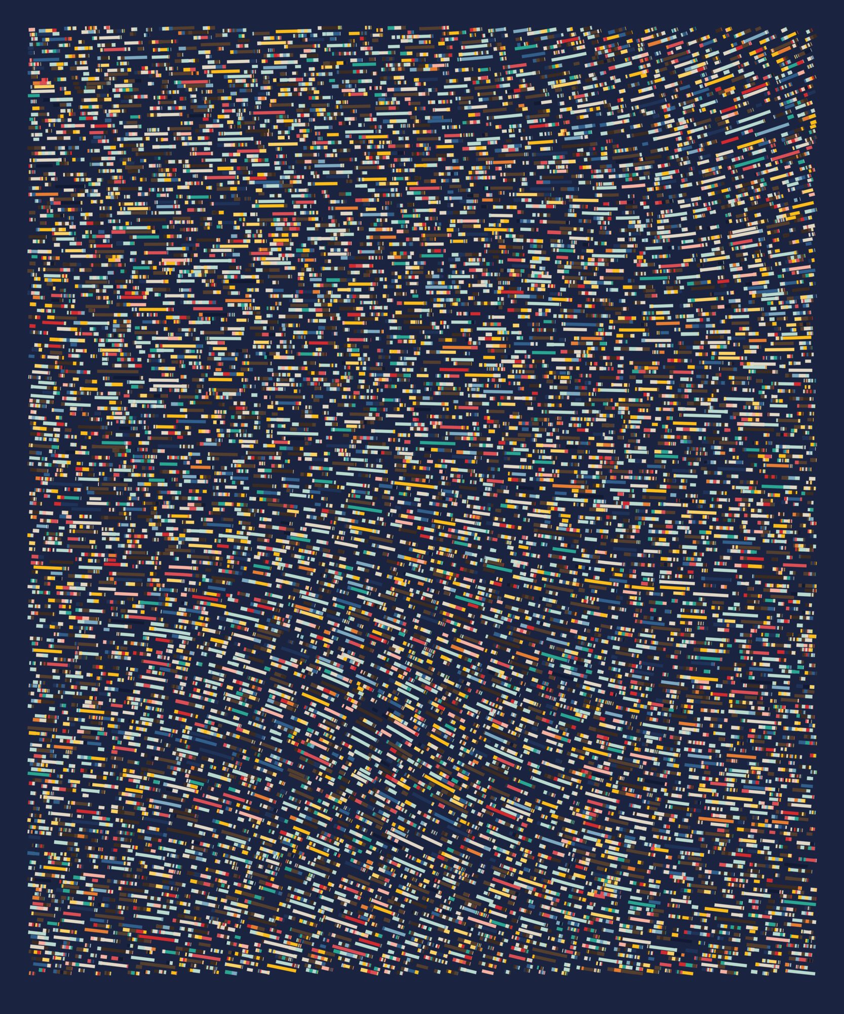
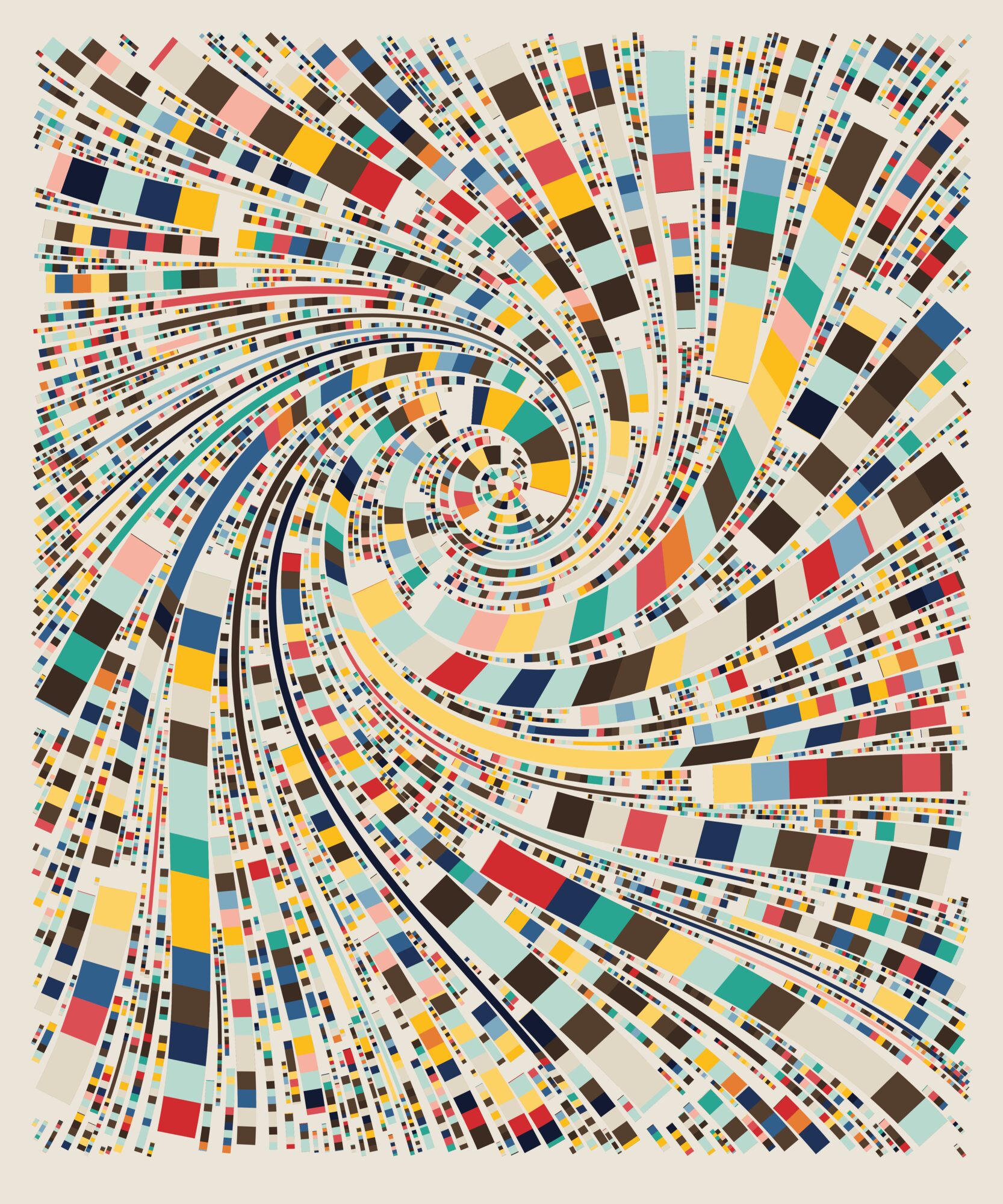
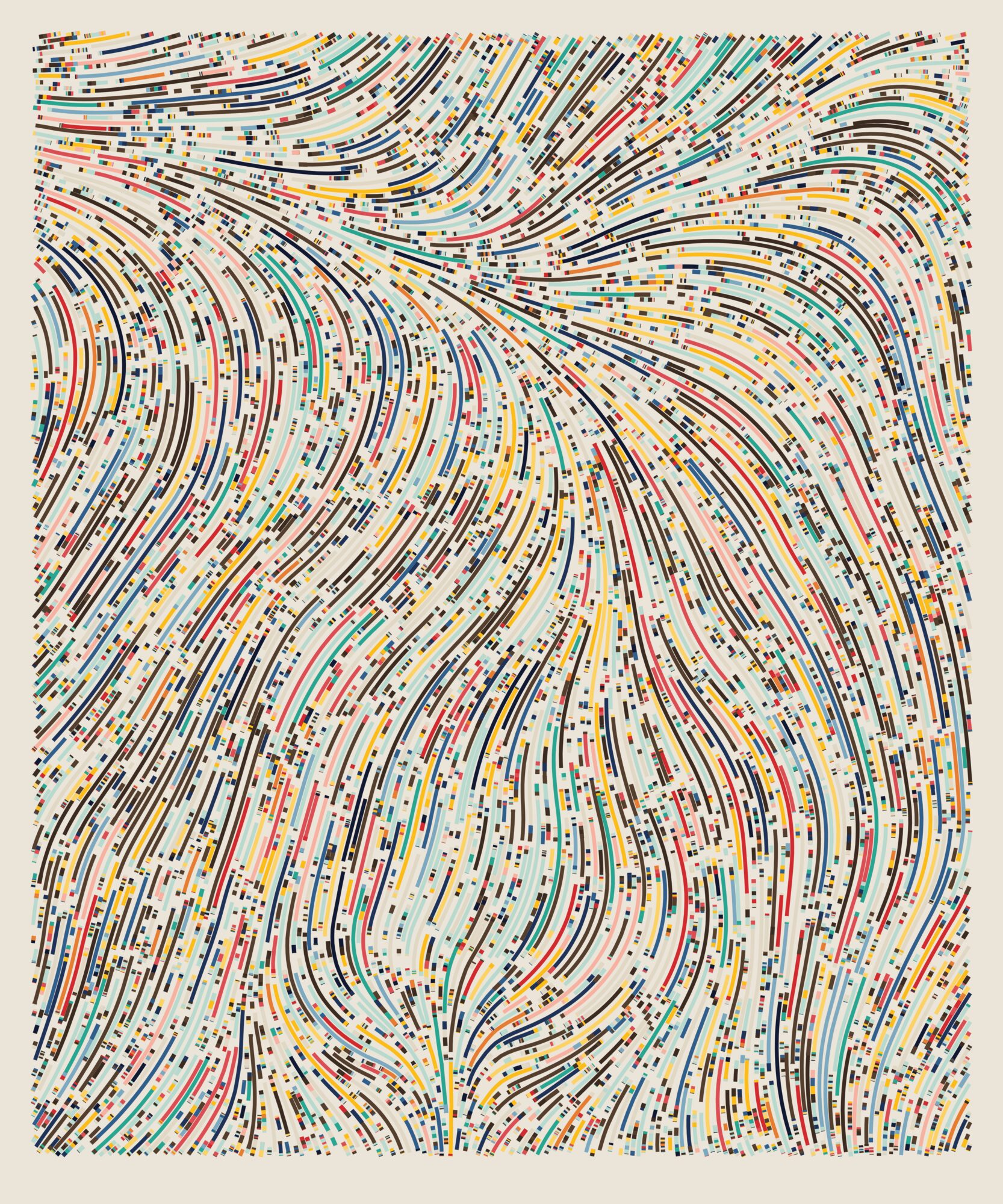
Also, Tyler sent me this `ArtBlocks’ link to his work: Fidenza on ArtBlocks
Out of boredom, or perhaps the useful kind of boredom that comes when the mind has no obvious administrative object to attach itself to, I started wondering whether one could quantify some of those rules. Could one extract a mathematical principle from the visual family rather than merely describe its traits? Not the color palette, not the nominal size categories, but something about how rule, scale, and visible complexity were related.
The click !
That is when the Chaitin thread and the Fidenza thread clicked together.
In Chaitin’s metabiology, scale is not a matter of visual size. It is a scale of complexity: how much algorithmic information is present, how much can be specified, how far a formal or evolutionary process can climb. In Fidenza, scale is visual and geometric, but it also changes the apparent information density of the work. A “jumbo” piece can look simple because the canvas is organized by a few large structures. A dense micro-scale piece can look as if far more computation has been packed into the same bounded surface. The canvas has not changed. The rule has not become a different physical world. What changes is the relation between the rule and the scale at which its consequences are made visible.
That was the bridge to neurons.
The point neuron is one of the great abstractions in theoretical neuroscience. It has earned its place. Treating a neuron as a unit with inputs, a state variable, and an output has made enormous parts of neural network theory possible. It underlies models of recurrent dynamics, balanced networks, population computation, and much of modern NeuroAI. But a biological neuron is not literally a point. It has dendrites, branches, synapses, local nonlinearities, conductances, and spatially organized input. It is not a single computational degree of freedom before we choose to describe it that way.
The question that began to form was therefore not: are point neurons useful? Of course they are. The question was: what kind of projection has taken place when a spatially structured biological object is represented as a point?
Once stated that way, the problem became an information-theoretic one. If a detailed object is viewed through a coarse ruler, some information survives and some is lost. But more subtly, the structure of the surviving information can change. A dependency that is higher-order at one scale can appear pairwise at another. A mechanism that is nonlinear in the contact-level variables can look direct after those variables have been collapsed into a somatic or population-level observable. Conversely, a model can predict very well at the coarse scale while being silent about the finer computation that generated the variables it uses.
This is the core of the paper. The coastline paradox says that the length of a coast is not a property of the coast alone; it is a joint property of the coast and the ruler. I wanted to ask the analogous question for neural computation. How long is the coast of a neuron? More precisely: how does the apparent order, directness, sparsity, and computational capacity of a neuron change when the ruler changes from contacts, to branches, to soma, to population activity?
The framework that came out of this separates several quantities that are often verbally blurred together. At a given resolution, how much predictive information about the output is available at all? How much of that information can be captured by a direct model? How much remains as a residual outside the direct family? Coarse-graining cannot increase the total information available, by data processing. But it can change the apparent order of the information that remains. It can erase distinctions needed to see a nonlinear interaction. The coarse description can therefore look more direct precisely because the relevant microscopic distinctions have been removed.
That is the “denominator trap” in the paper: a direct fraction can rise as the total surviving information falls. A model can look closer to perfectly direct at the coarse scale not because the underlying mechanism has become simple, but because the ruler has discarded the degrees of freedom that would have revealed the complexity.
The later timing of the project became unexpectedly fortunate. A recent paper by Christopher Lynn in Nature Physics argued that simple input-output dependencies explain a large fraction of neuronal activity. The result generated a strong reaction among neuroscientists. Some saw it as evidence that low-order or direct descriptions may be much more powerful than expected. Others objected that such models could not settle the underlying cellular or circuit mechanism. Safaai and Sabatini, for example, pushed on the identifiability problem from another direction: when a model attributes activity to direct dependencies, how stable is that attribution under changes in the sampled input distribution?
This debate made the scale issue unavoidable. My paper is not simply an argument against Lynn’s result, nor is it a dismissal of the objections to it. I think the more interesting point is that both sides are looking at real aspects of the same problem. A successful direct model is a real fact about a system at a declared scale, under a declared distribution, using a declared family of models. But it is not automatically a mechanistic identification of the computation beneath that scale. Predictive adequacy and mechanistic identification are two sides of one moon. The missing piece is the map between rulers.
That is why the biophysics matters. The paper is not trying to float an abstract information-theoretic objection above the cell. Dendrites give the problem its physical content. Local voltage, conductance, driving force, NMDA nonlinearities, branch saturation, electrotonic attenuation, and somatic mixing are not decorative details. They are the actual operations through which a contact-level computation becomes a branch-level signal and then a somatic variable. The point neuron is the weak-input, coarse-ruler limit of a richer physical object. It is a regime, not the identity of the cell.
This also changes how I think about NeuroAI. A standard artificial unit is closer to a point-neuron abstraction than to a biological neuron. A pyramidal cell, with its dendritic subunits and local nonlinearities, is closer to a small network whose internal architecture has been compressed into one biological unit. If we compare artificial networks and brains only at the level of point units, we may be comparing the wrong objects. Some computation can be allocated between units; some can be allocated within units. Which scale we choose determines which possibilities are even visible.
In retrospect, the path from Chaitin to Fidenza to neurons was not as strange as it first sounds. Chaitin forced the question of information scale. Fidenza made vivid how hidden rules become visible differently at different scales. The pandemic made projection itself feel almost physical: a world of high-dimensional encounters flattened into surfaces. And the point neuron was sitting there in neuroscience as our most productive, most dangerous projection.
The paper came from trying to take that projection seriously.
Not to abolish it. Not to claim that the finest ruler is always the right one. A fine ruler can be costly, noisy, and unnecessary for a given question. But a ruler should be declared. If a point-neuron model predicts well, that is a statement about what is visible at the somatic or population scale. It does not by itself tell us how long the coast is at the dendritic scale, or which computations were folded into the point before the measurement began.
So the question “How long is the coast of a neuron?” is not a metaphor added after the fact. It is the origin of the paper. It asks what happens when a biological computation is measured with different rulers, and when we forget that the ruler was part of the measurement all along.
How long is the coast of a neuron?
What the resolution of a neuron model does to the computation you can see — and to the computation you can build.
TL;DR. A neuron’s apparent complexity depends on the ruler you measure it with. Coarsen the ruler (point neuron, scalar weights) and genuinely multiplicative dendritic computation can look additive — not because it went away, but because the states it depends on were merged. Refine the ruler (resolve dendritic subunits) and a plain linear readout gains approximation power without receiving a single extra bit of information. For NeuroAI the consequence is sharp: the computational unit is a choice of resolution, not a neuron count, and three well-placed nonlinear subunits did the work of forty generic hidden features in my experiments.
1. Every model of a neuron picks a ruler
Mandelbrot’s coastline paradox is a statement about measurement, not geography: a coastline’s length is a joint property of the shoreline and the stick you walk along it with. Shorter stick, more inlets, longer coast.
Neuroscience and AI both walk the neuron with a very long stick. The point neuron — weighted sum, nonlinearity, out — is the default unit of recurrent-network theory, of balanced-network theory, and of essentially every artificial neural network ever trained. It has earned that status. It is also a coarse ruler, and it is worth asking what a coarse ruler cannot see.
The prompt for this work was a striking empirical result: maximum-entropy fits in which direct, pairwise dependencies on a small set of recorded neurons account for over 90% of a target neuron’s output entropy in mouse recordings (and about 60% in C. elegans). Read one way, that says single neurons are nearly additive. Read another way, it says a coarse description is predictively adequate at the scale of the recording. The paper is about why those two readings are not the same thing, and what each implies for building neural networks.
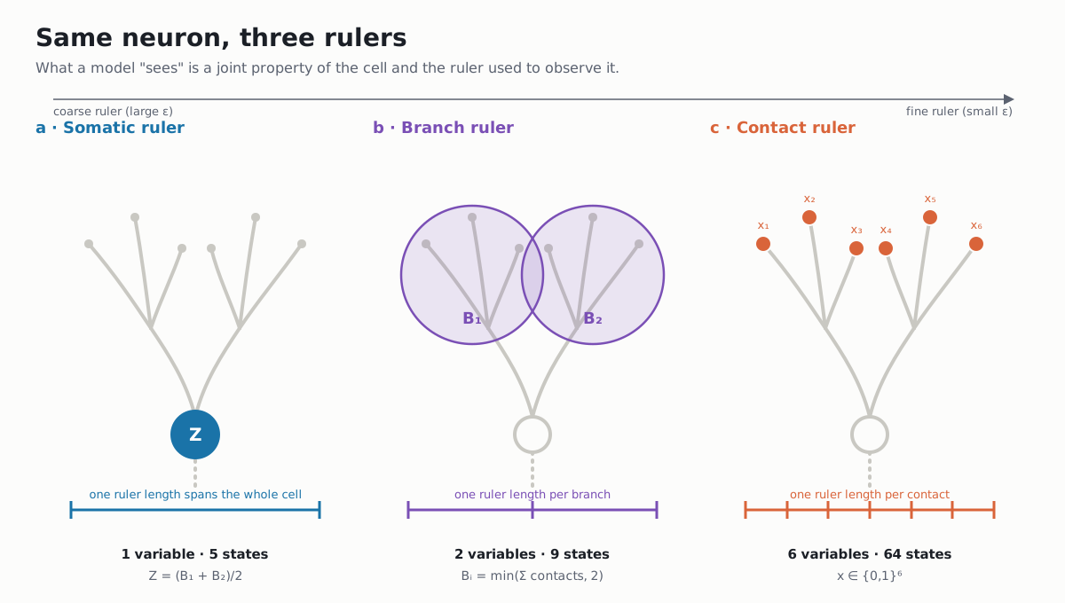
Figure 1. One neuron, three rulers. The somatic ruler sees a single variable; the branch ruler two; the contact ruler six. They are connected by many-to-one maps, and only one of them matches what a point-neuron ANN unit computes.
2. Keeping honest books: what “direct” means
To make “direct” precise, fix a resolution $\varepsilon$, call the visible inputs $\mathbf X_\varepsilon$ and the output $Y$. The direct family is every model of the form $\sigma[b + \sum_i u_i(x_i)]$ — any function of each input on its own, no joint terms. Fit the best member of that family and the output uncertainty splits into three non-negative pieces:
\[I_{\text{avail}} \;=\; I_{\text{dir}} \;+\; I_{\text{higher}},\]where $I_{\text{avail}} = I(Y;\mathbf X_\varepsilon)$ is everything the inputs could tell you at this ruler, $I_{\text{dir}}$ is the part the best additive model captures, and $I_{\text{higher}}$ — which turns out to be exactly a conditional KL divergence between the truth and the best direct fit — is what demands joint terms.
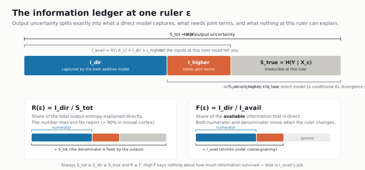
Figure 2. The ledger at one ruler, and the two ratios people quote.
Two ratios follow. $R = I_{\text{dir}}/H(Y)$ is the share of total output entropy that is direct — the max-ent number. $F = I_{\text{dir}}/I_{\text{avail}}$ is the share of available information that is direct. They look interchangeable and are not: $R$’s denominator is pinned by the output, while both parts of $F$ move when the ruler changes. That asymmetry is the whole story.
3. A coarser ruler can make a neuron look simpler
Projecting fine variables onto coarse ones can only lose predictive information (data processing). What it does to the structure of the survivors is not constrained at all. Two exact constructions make this concrete.
Order is not invariant. Take three spins coupled only through a three-body term, $P\propto\exp(K s_1 s_2 s_3)$. Every pair marginal is flat, so a pairwise model sees nothing; the entire dependence is third-order (0.823 bits at $K=1.8$). Now keep only $x = b_1$ and $z = b_2 \wedge b_3$: the ordinary mutual information between these two coarse variables is 0.261 bits. Keep $z = \mathbb 1[b_2=b_3]$ instead and it is the full 0.823 bits. Nothing was added; a many-to-one map re-expressed existing third-order structure as pairwise.
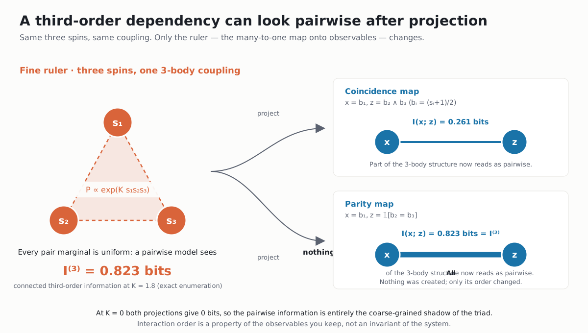
Figure 3. The order at which a dependency appears belongs to the observables you keep, not to the system.
The denominator trap. Now a neuron-shaped version. Six binary inputs feed two three-input dendritic subunits, and the output fires strongly only when a whole triplet is co-active — a cartoon of NMDA-type coincidence detection. Follow that fixed law through three rulers, all 64 input states enumerated exactly:
| ruler | observable | states | $F$ (direct share) | $I_{\text{avail}}$ (bits) |
|---|---|---|---|---|
| contacts | $\mathbf x\in{0,1}^6$ | 64 | 55% | 0.157 |
| branches | $B_i = \min(\text{active in branch } i,\,2)$ | 9 | 96% | 0.029 |
| soma | $Z=(B_1+B_2)/2$ | 5 | 100% | 0.024 |
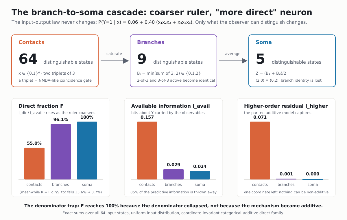
Figure 4. Saturation merges “two active” with “three active” — the exact distinction the coincidence gate depends on. Averaging then merges the two branches. The direct share climbs to 100% while 85% of the predictive information is discarded and the higher-order residual collapses to zero.
The neuron is “more direct” at each step for one reason: the observer can no longer tell apart the states on which the interaction lives. Meanwhile $R$ falls (13.6% → 3.7%). A high $F$ with a shrinking $I_{\text{avail}}$ is not evidence of an additive mechanism — it is evidence that the ruler got longer. Two sanity checks in the paper: the direct family must be categorical (forcing branch states onto a line fakes a residual), and an asymmetric somatic mixture ($0.6B_1 + 0.4B_2$) keeps branch identity recoverable and drops the linear direct share from 99% to 78%. “Directness” is a property of the whole measurement pipeline, not of the cell.
4. A weight is a compressed field
The most basic object in any network model inherits the same issue. At neuron resolution a connection is one scalar $w_{ij}$. At contact resolution the same connection is a field of synapses on different branches, each read in a local state (local voltage, Mg²⁺ block, what the neighbours are doing). The scalar is the output of a projection applied to that field, and the projection obeys the data-processing inequality like any other.
So anatomical directness and informational directness come apart. A connection can exist ($A_{ij}=1$) and still fail to contribute additively, because its effect depends on the dendritic context it lands in. One line captures it:
\[\operatorname{logit}P(Y=1\mid x_j,n) = b + \alpha x_j + \beta n + \gamma\, x_j n .\]Same anatomy for every $\gamma$; informationally direct only when $\gamma=0$.
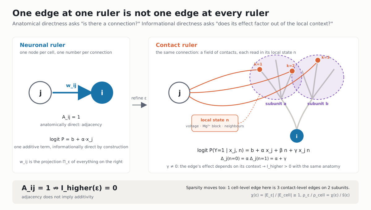
Figure 5. One edge at the neuronal ruler is a context-dependent contact field at the contact ruler. Adjacency does not imply additivity.
| For NeuroAI this bites twice. An ANN weight is informationally direct by construction — it has no local context to depend on — so an architecture built from scalar weights has already committed to the coarse ruler before training starts. And when a connectome is translated into a network, collapsing contact-level edges to cell-level edges changes sparsity, degree and density (the compression factor $\chi(\varepsilon)= | E_\varepsilon | / | E_{\text{cell}} | $ is at least 1 and can be large). A graph that is sparse axon-to-cell can be dense contact-to-subunit, and that denser graph is where the nonlinear features live. |
5. A finer ruler buys capacity, not information
Now the reverse direction, and the part aimed squarely at architecture design. Resolving dendritic subunits does not change the target function or the information available about it; it changes the feature space a readout can draw on. I tested this with held-out regression on a target with known pairwise and triple interactions over six centered inputs.
Organization beats count. A linear point neuron reaches held-out MSE 0.044. Give each input three contacts grouped into three nonlinear subunits aligned with the target’s pair structure: 0.031. Same 18 contacts, same three subunits, contacts shuffled: 0.039. Exposing nonlinearity helps; placing it where the computation is helps more. A generic network of fixed sigmoid random features needs 40 units to match the three aligned subunits.
Resolution as a dial. To isolate resolution itself, draw one 24-subunit sigma–pi architecture and expose its first $n$ subunits to a linear readout. Because every feature set is a deterministic function of the inputs, $I(Y;\Phi_n)$ is identical for all $n$ — refinement adds zero information — yet the hypothesis class is strictly nested and held-out error falls monotonically (0.042 → 0.015), scaling as $n^{0.31}$. The participation ratio of the feature covariance, a label-free effective rank, rises from 6.9 to 14.0, scaling as $n^{0.24}$. The new coordinates span new directions; they are not duplicates.
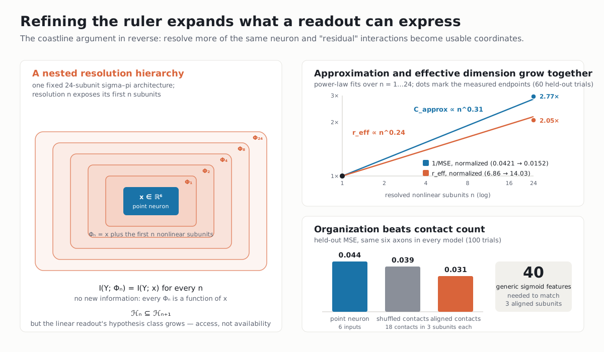
Figure 6. Access, not availability. Exponents describe this construction, not a biological law.
6. What this means for NeuroAI
Putting the two directions together gives a set of design and interpretation rules I think are under-appreciated.
The unit is a resolution, not a neuron. “Biologically plausible” networks are often specified by matching cell counts or cell-level connectivity. Neither fixes the computation at a node. The question that does is: which contact groups, nonlinear features and state dependencies does each unit retain? Three aligned subunits ≈ forty random features is the kind of exchange rate that answer sets.
Multiplicative structure is cheap when it is local. Coincidence detection, saturation and context-gated synapses are all forms of $x_j n$ terms. A point unit has to synthesize those from width; a unit with resolved subunits gets them as coordinates. This is the biophysical argument for sigma–pi, gated, or dendrite-like units — not mimicry, but approximation economy.
Sparsity has to be stated with its graph. Pruning, lottery tickets and connectome-constrained models all quantify sparsity on a cell-level graph. The same system can be far denser at the subunit level, and the subunit level is where the usable nonlinear features are. Compare sparsity across models only at matched resolution.
Probes are rulers too. A linear probe on hidden activations, or a pairwise model fitted to recorded units, is a coarse ruler applied to a network. A high direct fraction tells you the probe’s coordinates suffice for that readout under that input distribution. It does not tell you the mechanism is linear, and a vanishing residual can mean the interesting states were merged, not that they were absent. Report $I_{\text{avail}}$ alongside $F$, and perturb the input distribution before calling a representation “simple”.
Bounds are real, and they are scale-indexed. A fit with $R>0.9$ does bound what any unobserved variable can add to predicting that output under that state distribution — at most $(1-R)H(Y)$. That is a useful guarantee. It is a statement about a readout, not about dendrites.
7. So how long is the coast?
Like the coastline, the question is well posed only after four things are fixed: the ruler (which variables are resolved), the target observable (spikes, branch voltage and plasticity each want a different adequate resolution), the class of perturbations you will test adequacy against, and the domain of conditions over which you claim it. Hold the output fixed, ask how much finer variables add, perturb, repeat. Continued success validates the reduction inside that domain and nowhere else.
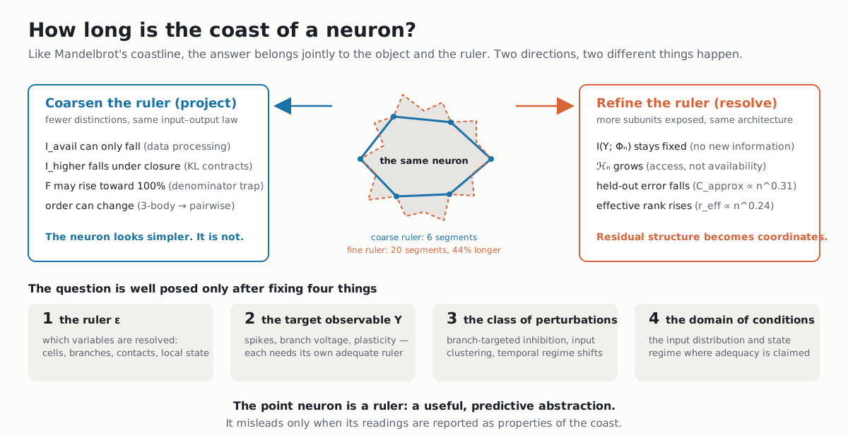
Figure 7. Coarsening hides; refining exposes. Neither direction creates or destroys the neuron — only the description.
The point neuron is a ruler. It is a good one, and most of deep learning is built on it. The mistake is not using it; the mistake is reporting its readings as properties of the coast — and then designing the next generation of networks to match the readings instead of the coast.
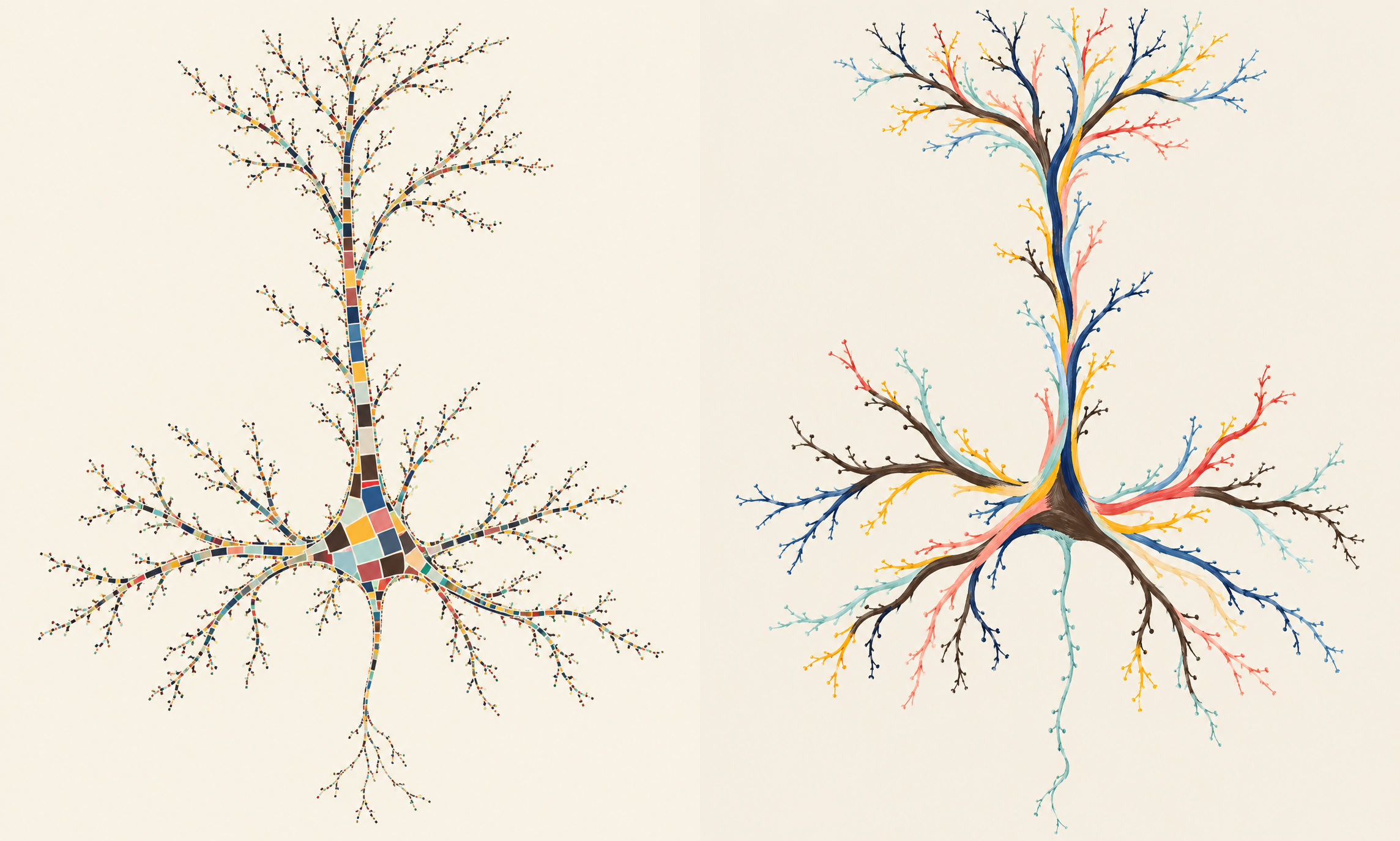
NeuroFidenza!
Cite this post
@misc{dehghani2026CompRes,
  author       = {Nima Dehghani},
  title        = {{What the resolution of a neuron model does to the computation}},
  year         = {2026},
  howpublished = {\url{https://neurovium.science/posts/pblog-CoastOfNeuron/}},
  note         = {Companion post to: How Long Is the Coast of a Neuron? Resolution-Dependent Interaction Order and Computational Capacity (2026). doi:10.48550/arXiv.2610.19487}
}