The Silhouette Fallacy: Field closure, ephaptic coupling, and the physics of computation
Companion post to:
Field closure, ice neurons, and when a dendrite is a motif
Nima Dehghani
arXiv 2026
DOI: https://arxiv.org/abs/2610.00184v1
@misc{dehghani2026SilhouetteFallacy,
  author       = {Nima Dehghani},
  title        = {{The Silhouette Fallacy}},
  year         = {2026},
  howpublished = {\url{https://neurovium.science/posts/pblog-IceNeuron/}},
  note         = {Companion post to: Field closure, ice neurons, and when a dendrite is a motif
                  (2026). doi:10.48550/arXiv.2610.00184}
}
The Silhouette Fallacy
Field closure, ephaptic coupling, and the physics of computation
Companion to “Field closure, ice neurons, and when a dendrite is a motif.”
A frozen pond can draw a neuron.
That sentence is both the beginning of the paper and the problem the paper is trying to solve.
Contents
- Origin — How this paper came to be · Walden in winter · The other Claude · Mullins–Sekerka: home at last
- The distinction — The silhouette fallacy · Ice is not pretending to be a neuron · The missing state · The neuron writes the field
- Closure in the model — Why closure rather than feedback? · One knob deforms the physics · Freeze the tree · The graph is not the whole architecture
- What it means — Three possessions · The physical-computing lesson · The NeuroAI lesson · The fallacy, in one sentence
How this paper came to be
The story behind this paper is part serendipity and part a sequence of past encounters with the right people at the right time.
The serendipity was ice.
The rest had been accumulating for years.
Walden in winter
The random encounter with the pond neuron happened on a winter day while I was walking around Walden Pond — yes, that Walden Pond, the one made famous by Henry David Thoreau.
I had always loved Walden. It is an astonishingly tranquil place. Years ago, outside the summer season, there were days when it felt almost empty. Over the past decade it has become much more of a destination; in summer it buzzes with families, swimmers, visitors, and people making the pilgrimage to Thoreau’s pond.
I still wanted my quiet walks.
So one winter day, while I was thinking about physical computing and closure, I went there precisely because winter more or less guarantees that you will not bump into many other people.
Instead, I bumped into something much stranger.
We have all seen branching structures. Arteries. Bronchioles in the lung. River networks from an airplane. Tree canopies. Cracks. Lightning. Branching itself is not surprising.
But these were different.
Under patches of snow-covered ice were dark branching formations with an uncanny similarity to neurons. Some looked multipolar. Some had a dark soma-like center with a long polarized arbor. Some appeared as whole fields of competing dendritic trees.
It was eerie, and completely captivating.
I immediately assumed there had to be a thermal explanation. The formations were appearing specifically beneath the snow-covered parts of the pond, so some local heat differential and melting process had to be involved. But at that moment the physics was secondary. I just wanted to see them properly.
No one was around. I went home, grabbed some rope and carabiners I had, came back, tied myself off to trees on shore, and got close enough to the ice to take a ridiculous number of photographs.
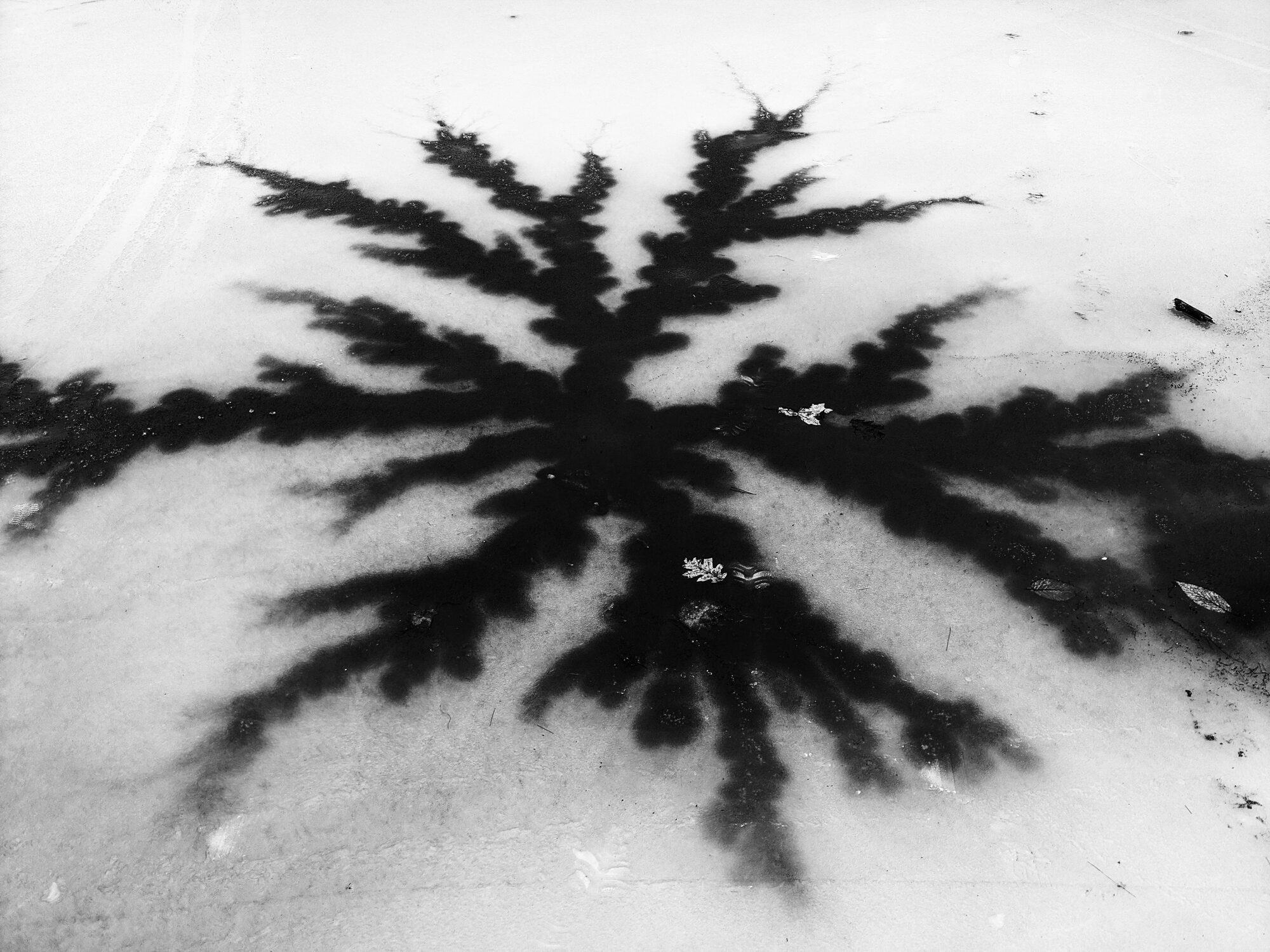
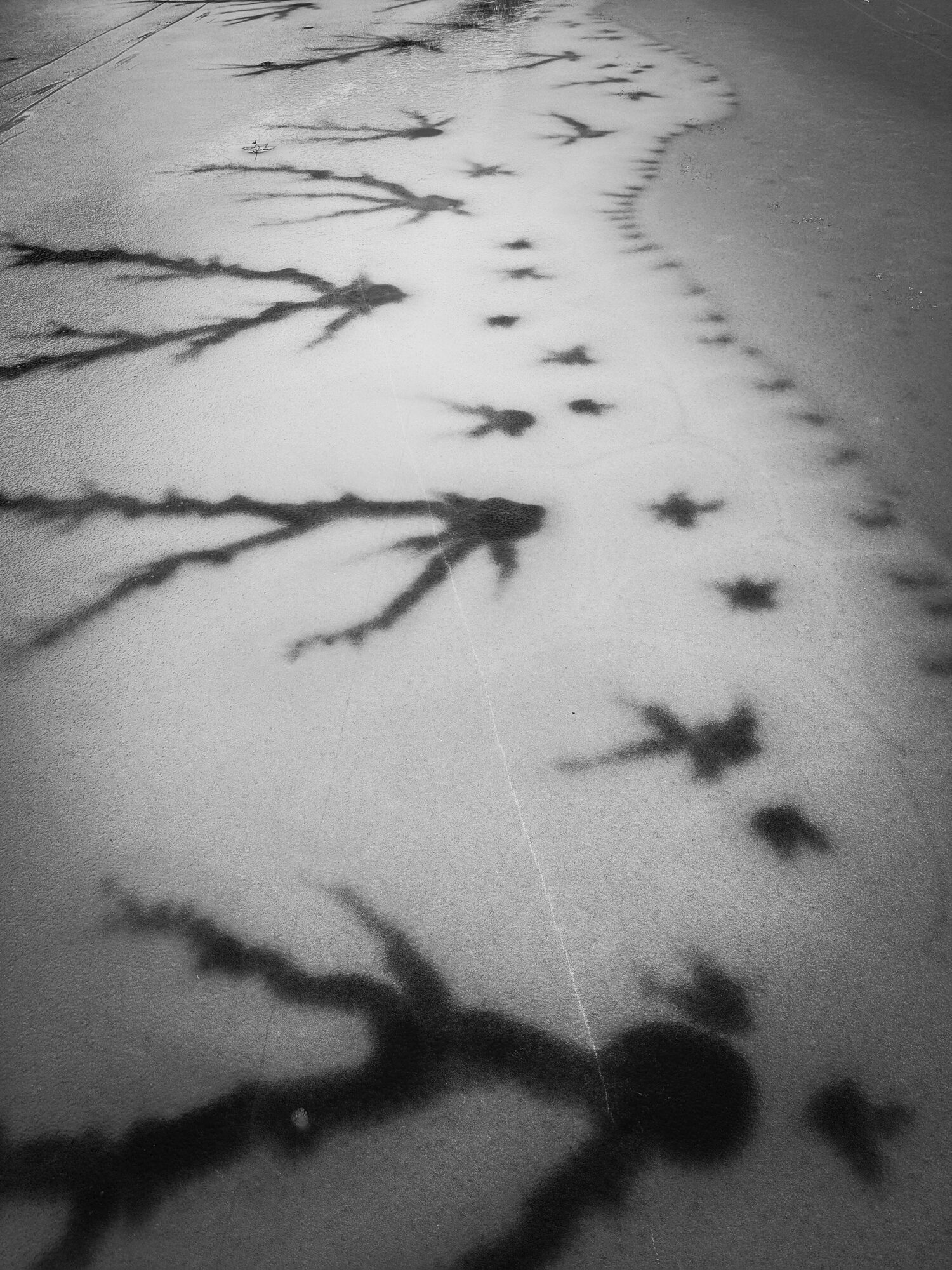
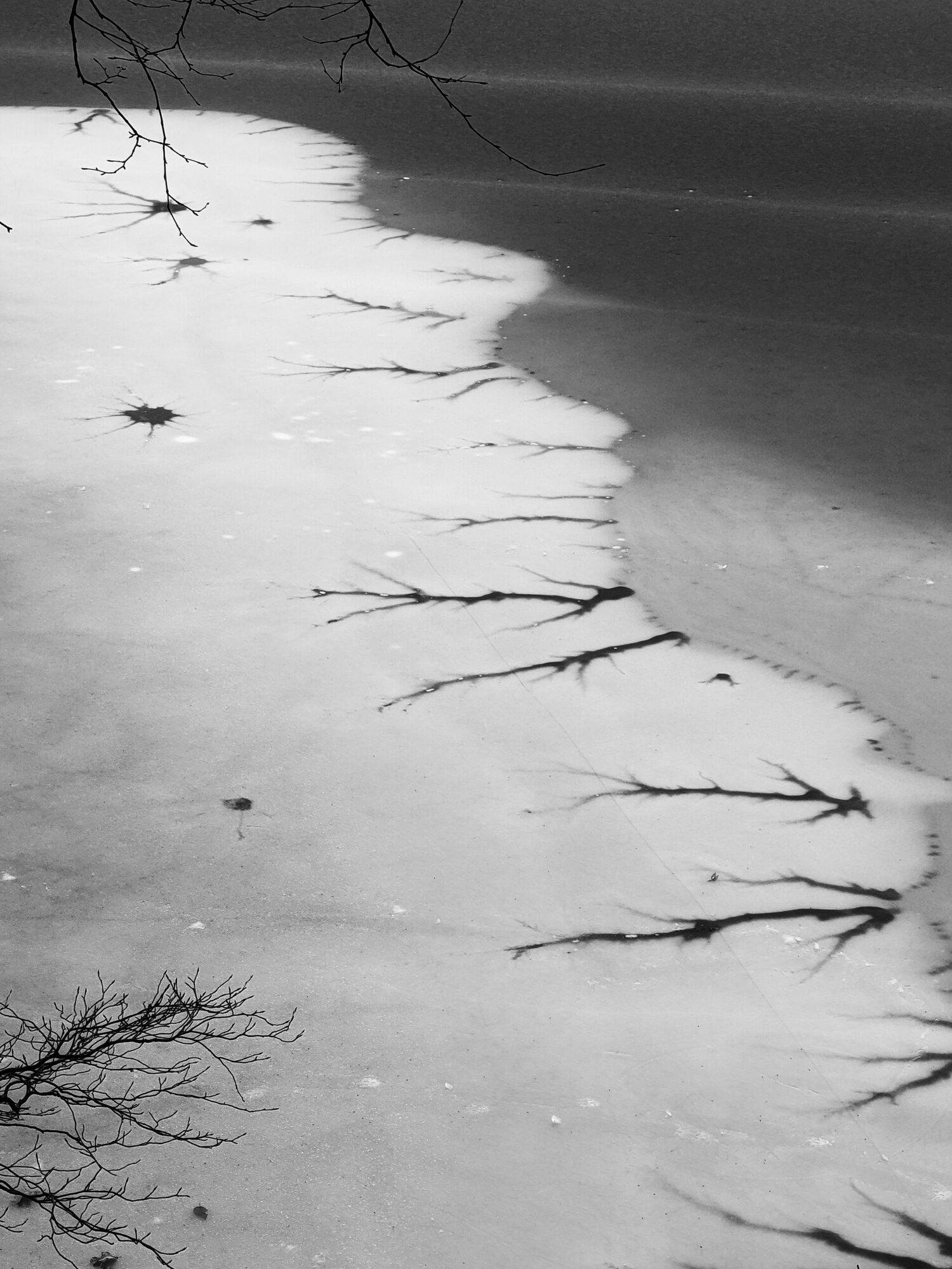
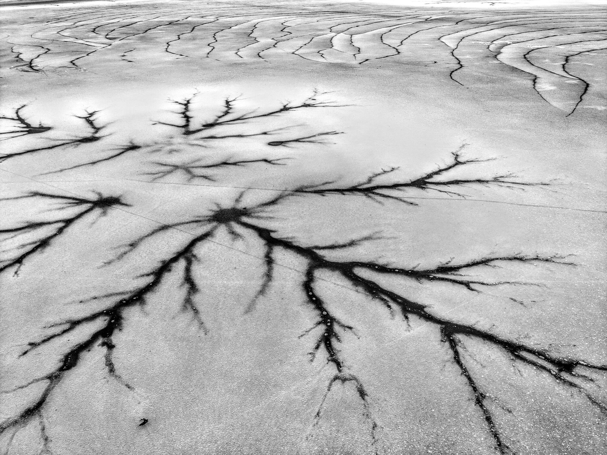
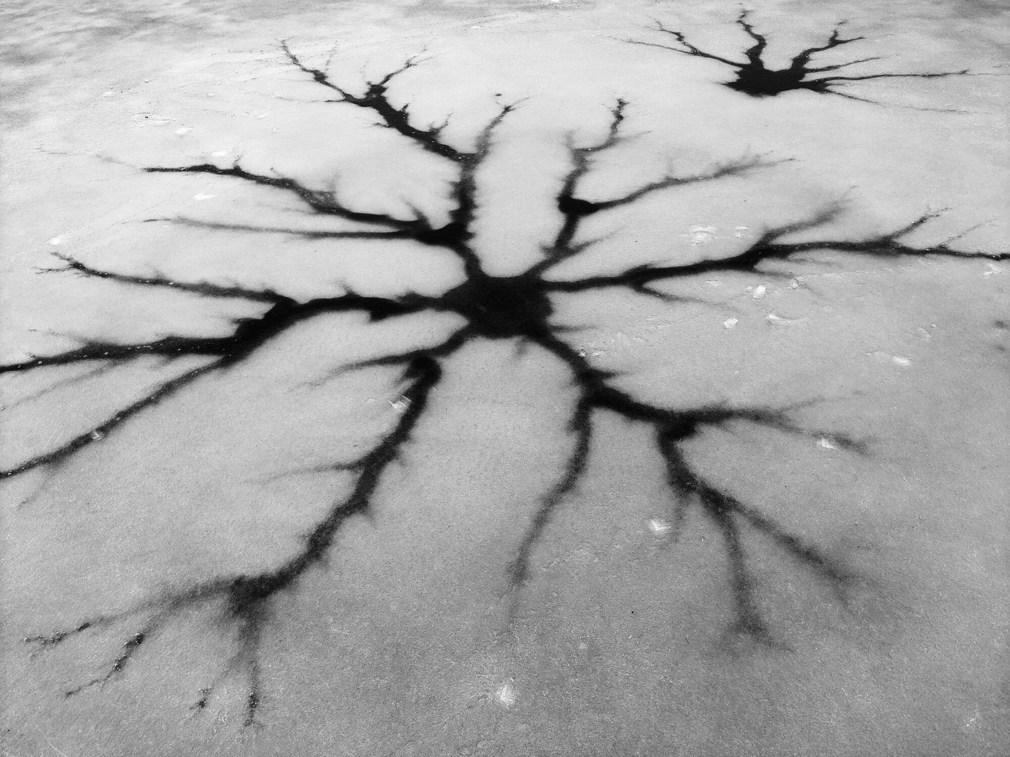
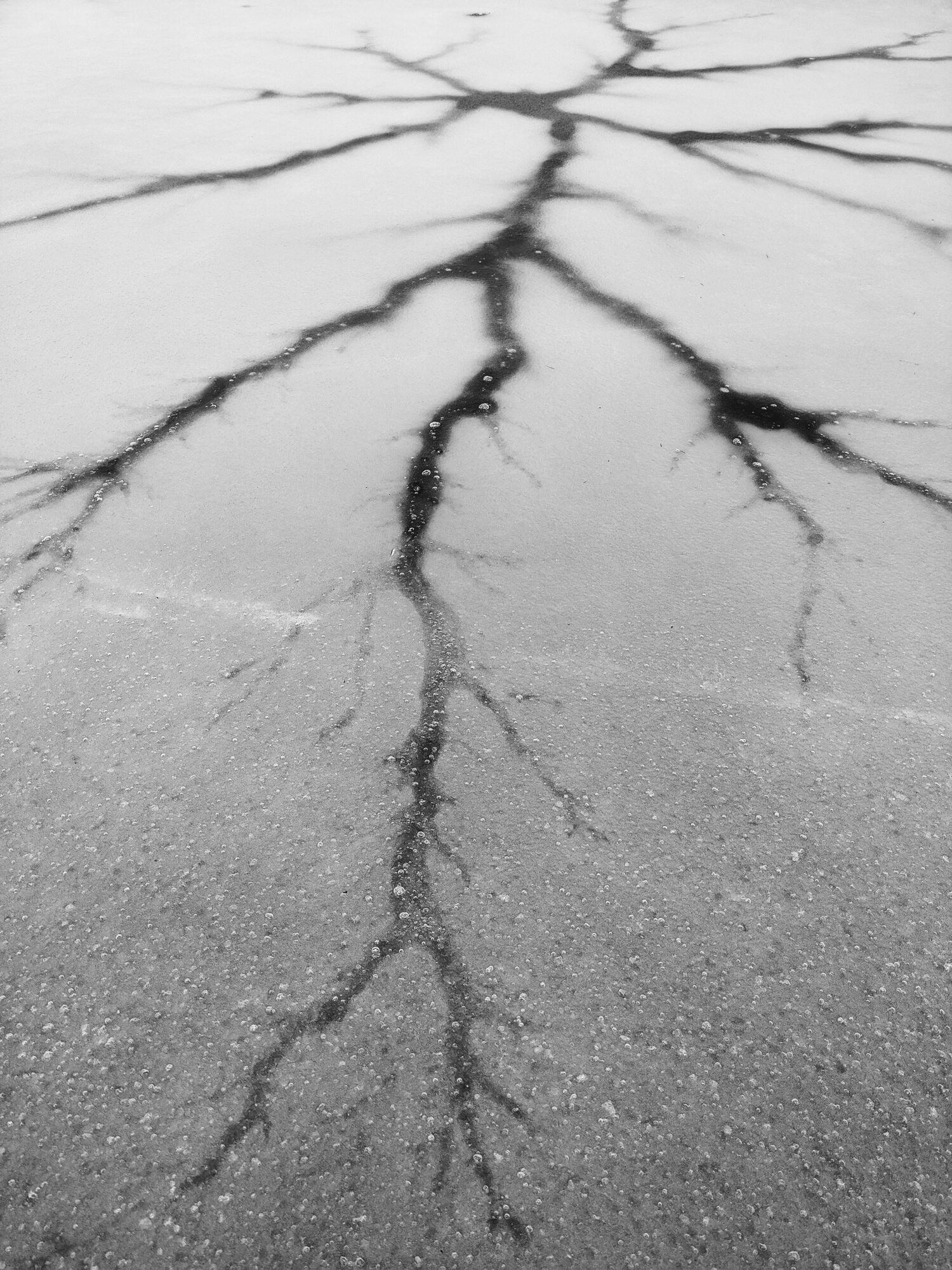
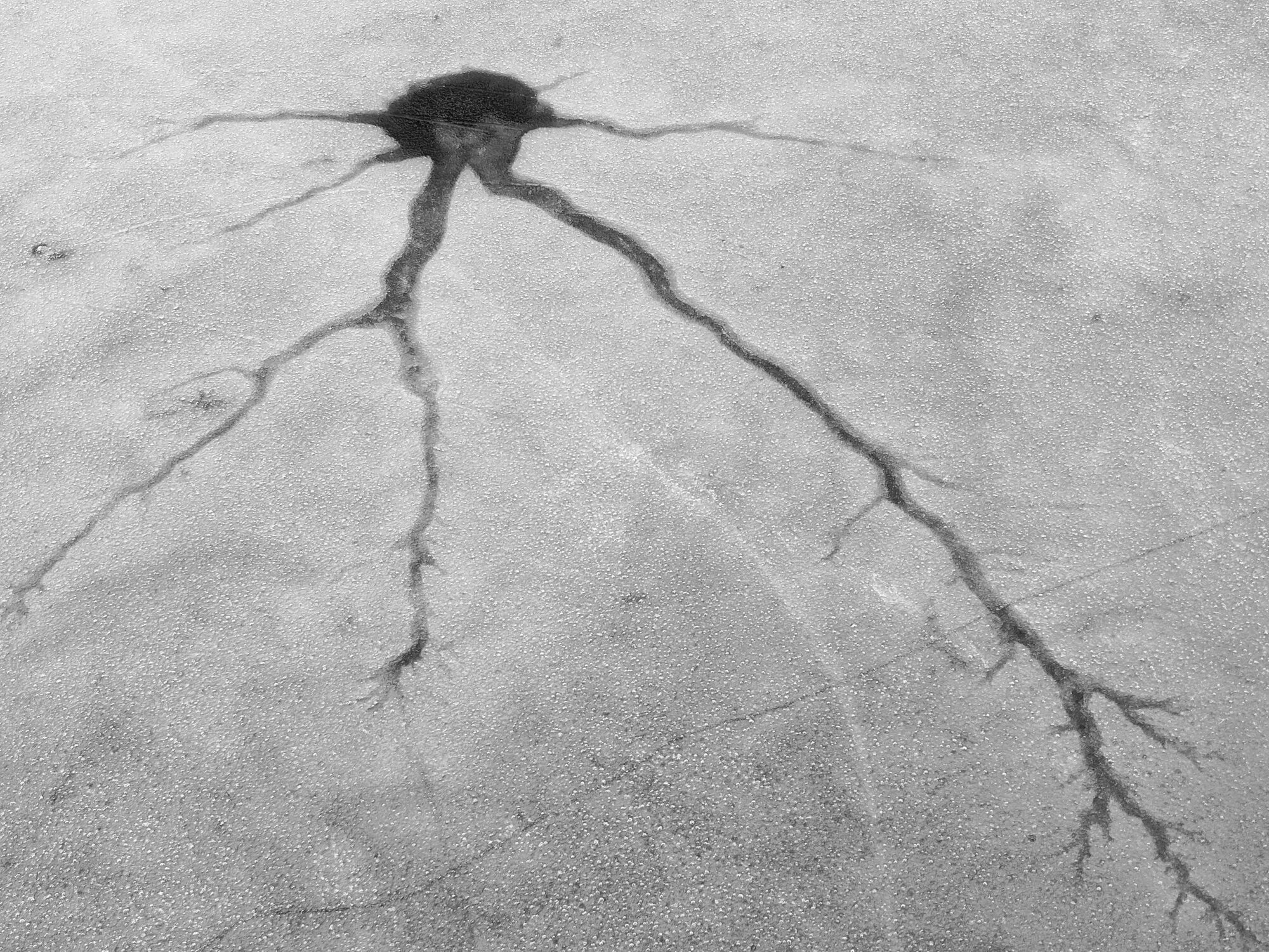
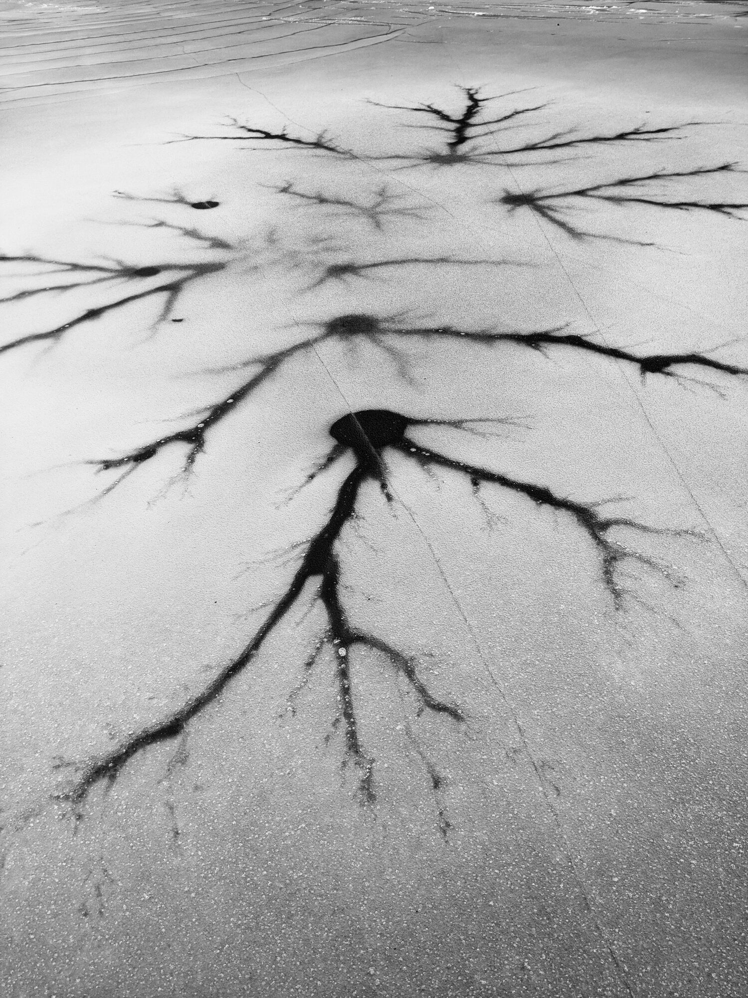
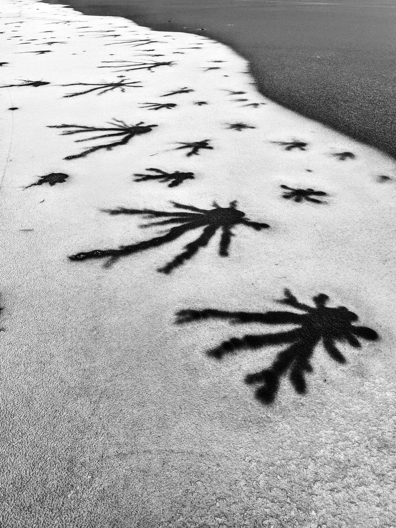
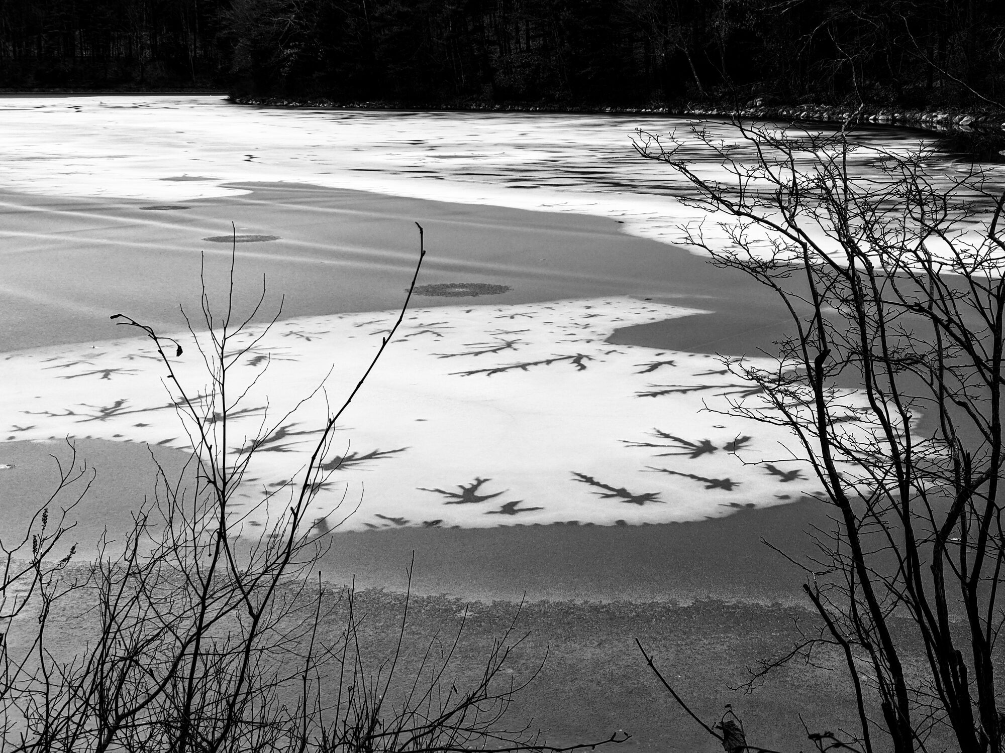
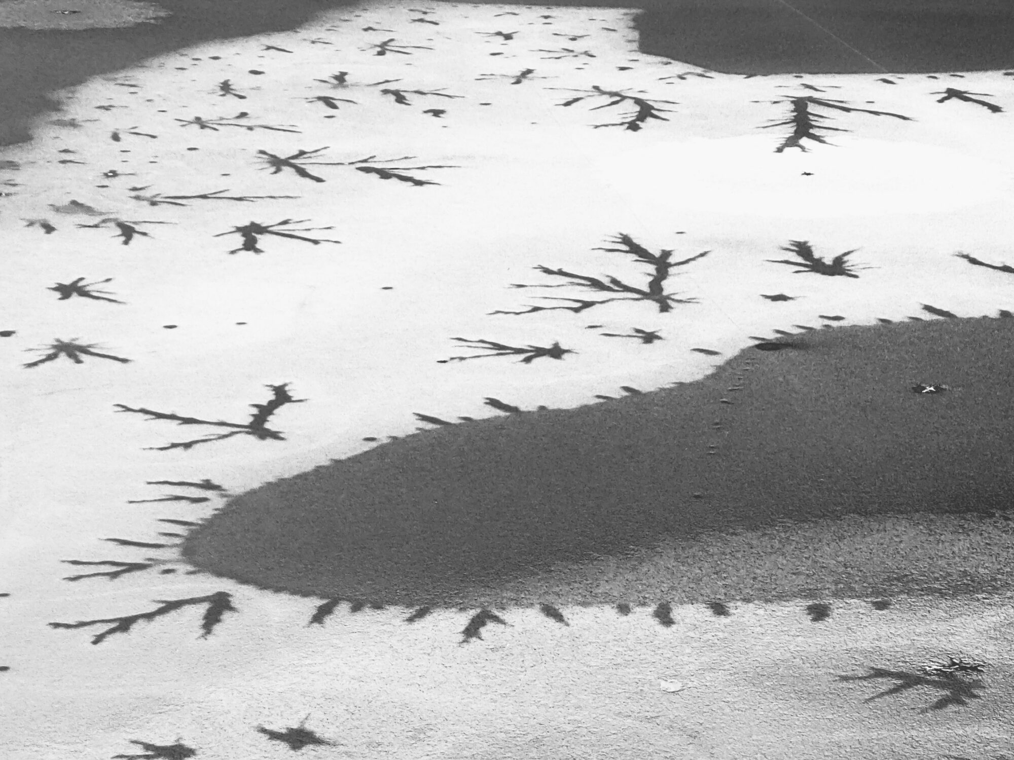
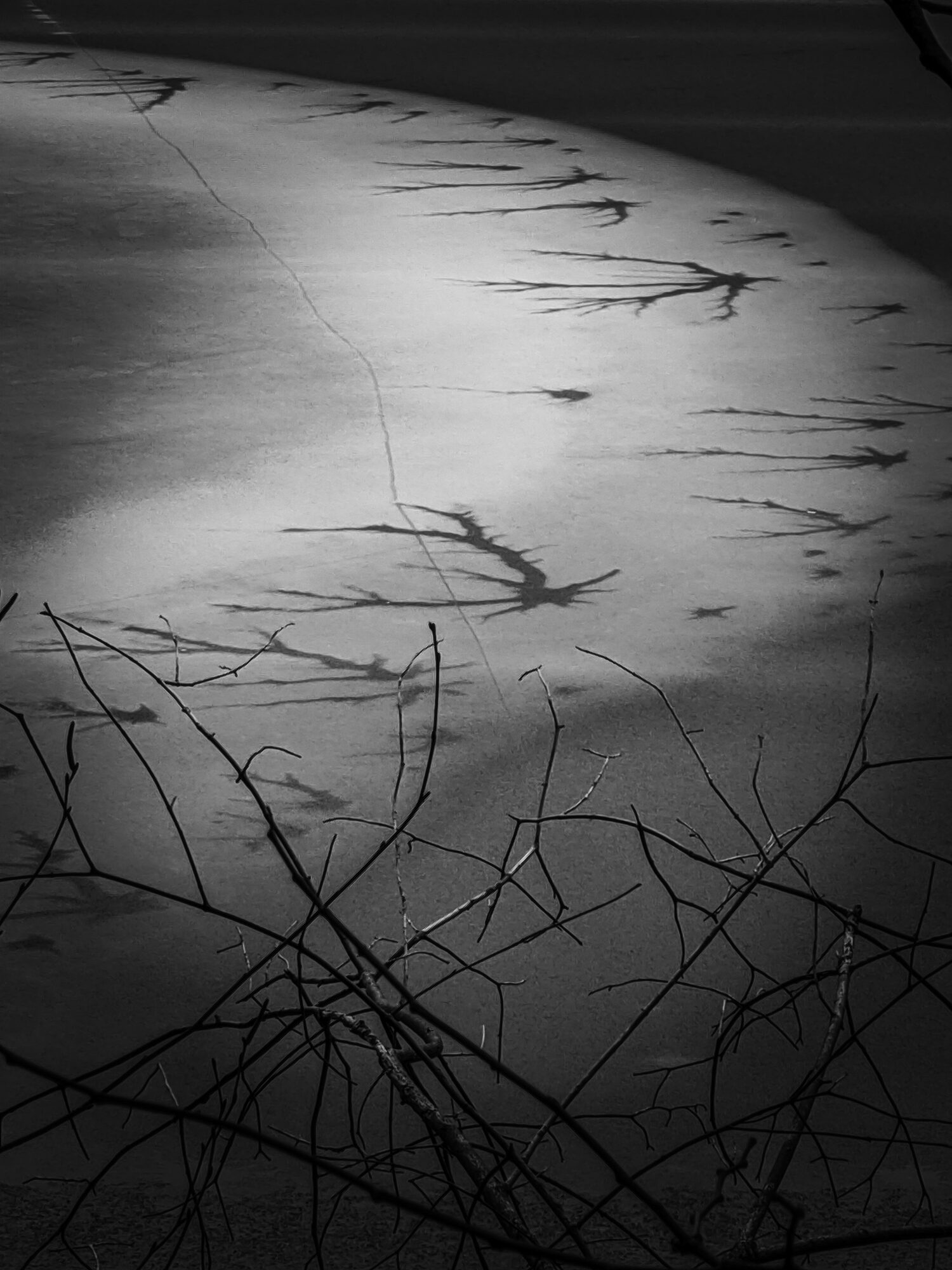
I started lining some of the ice neurons up next to one another, because once you have seen enough cortical anatomy it is almost impossible not to start making comparisons.
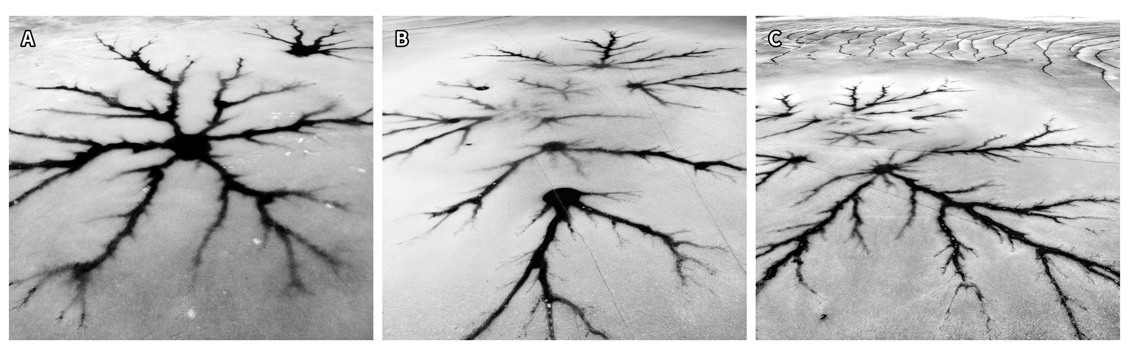
There is actually another paper hiding behind that 12th figure in the gallery. I have been working, on and off, on something about cortical columns,and how information and structure sculpt one another; but I still have not found the final bit of magic that makes the whole thing click. So for now it is in my drawer.
At this rate the drawer is turning into Professor Balthazar’s closet — if you ever saw that charming Croatian animation for kids, you know exactly the sort of place I mean: half laboratory, half cabinet of unfinished wonders, with some contraption in the back that may one day suddenly work.
And here is another photograph I particularly like, taken from farther away, where I was trying to get the branches of an actual tree and the branching ice formations into the same frame.
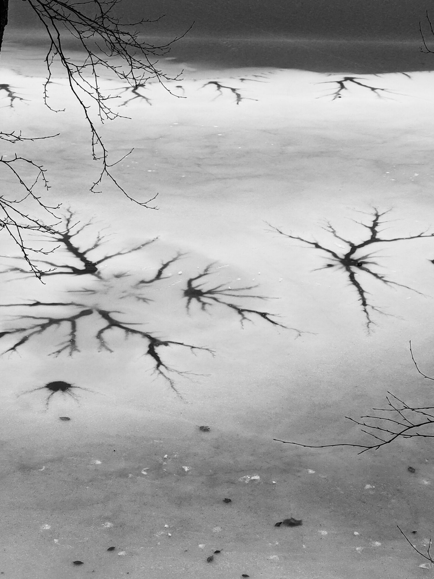
The whole thing fascinated me enough that I started searching around to see whether anyone else had noticed these structures.
Lo and behold: they had.
And, wonderfully, one of the reports was by a neurologist. Sandra Kostyk had published an image in Neurology under the title “Pond neurons.” (see Here!)
So I was not the first person to see the neuron in the ice (In fact, search for “Ice Neuron” in Google images and you will see numerous such examples by amused photographers).
But for me the interesting question was almost the reverse of what fascinated the neurologist.
The ice was obviously not a neuron. So why did it look so convincingly like one?
And what, exactly, was missing?
That made it a perfect negative control for something I had already been thinking about. In trying to understand information processing in biological systems, I had been circling around physical computing and closure: when does the physical substrate merely evolve, and when does its own internal state participate in organizing the operations we want to call computation?
And now there it was, staring at me from a frozen pond: a structure that had acquired the silhouette without acquiring the computation.
The other Claude
The other half of the story came from Claude.
No, not the Anthropic Claude.
A Québécois Claude! Claude Bédard.
A fine mathematical physicist, a very good classical guitarist, and a great chess player.
He’s the only one who’s ever beaten me twice in a row. I still carry that agonizing scar in my memory — even though I hold the better overall score against him.
Claude was an ex-teacher later turned research scientist in Alain Destexhe’s lab where I was doing my PhD with Alain. Alain himself came through the scientific lineage of Ilya Prigogine, and that mixture of nonlinear dynamics, statistical physics, biophysics, and neuroscience was simply the air of the lab.
At the time we were in Gif-sur-Yvette, on the CNRS campus outside Paris; a bit after I graduated, the lab moved to Saclay. Extracellular potential was bread and butter there. It was neurophysiology, biophysics, cable theory, and Maxwell’s equations all tangled together in exactly the way I liked.
With Claude and Alain I worked on my first PhD paper, on the scaling of extracellular sources in magnetoencephalography. Claude and Alain were also thinking deeply about cable theory and extracellular fields (you should read their paper!), and I had countless discussions with them: Claude smoking back-to-back cigarettes, all of us drinking a frankly unreasonable number of coffees, alternating between equations, neuroscience, physics, and sometimes chess.
What I learned from Claude was not one formula.
It was a way of moving.
He had this wonderful ability to jump from one physical concept to another through a chain of equations, never treating the mathematics as decoration. The equations were the road. You could begin with one physical statement and, if you followed the chain carefully enough, arrive somewhere that initially looked like a completely different subject.
From Alain, I learned to think about neuroscience as neurophysics in the deepest sense: to look for the organizing principles beneath the biological detail, with the nonequilibrium intuition of the Prigogine school always in the background.
That way of thinking became ingrained in me.
So years later, when I was staring at the ice neurons and thinking about field closure, the ingredients were already somewhere in my head: extracellular potentials are generated by neural activity; fields are physical variables, not merely observer-side readouts; cable dynamics lives on the morphology; and the extracellular medium gives you another route by which one part of the system can act on another. Ephatic coupling is not something that we can easily discount away.
I had the pieces.
I just did not know how to connect them.
And that annoyed the hell out of me.
Mullins–Sekerka: home at last
The connection finally arrived from a completely different direction.
One day I was reading parts of Michael Cross and Henry Greenside’s insanely good and intensely dense Pattern Formation and Dynamics in Nonequilibrium Systems.
And there it was:
Mullins–Sekerka instability.
Boom.
Home at last.
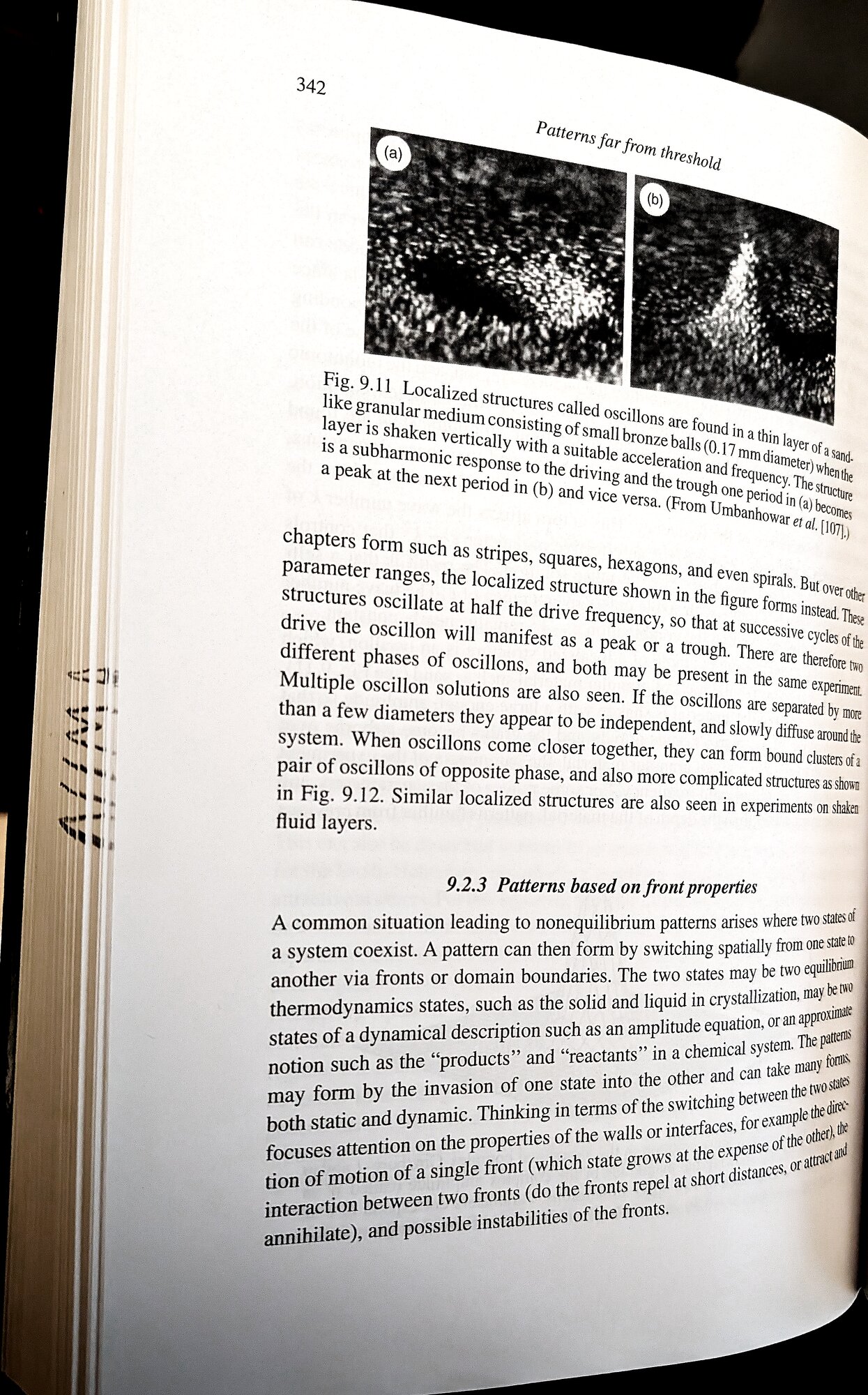
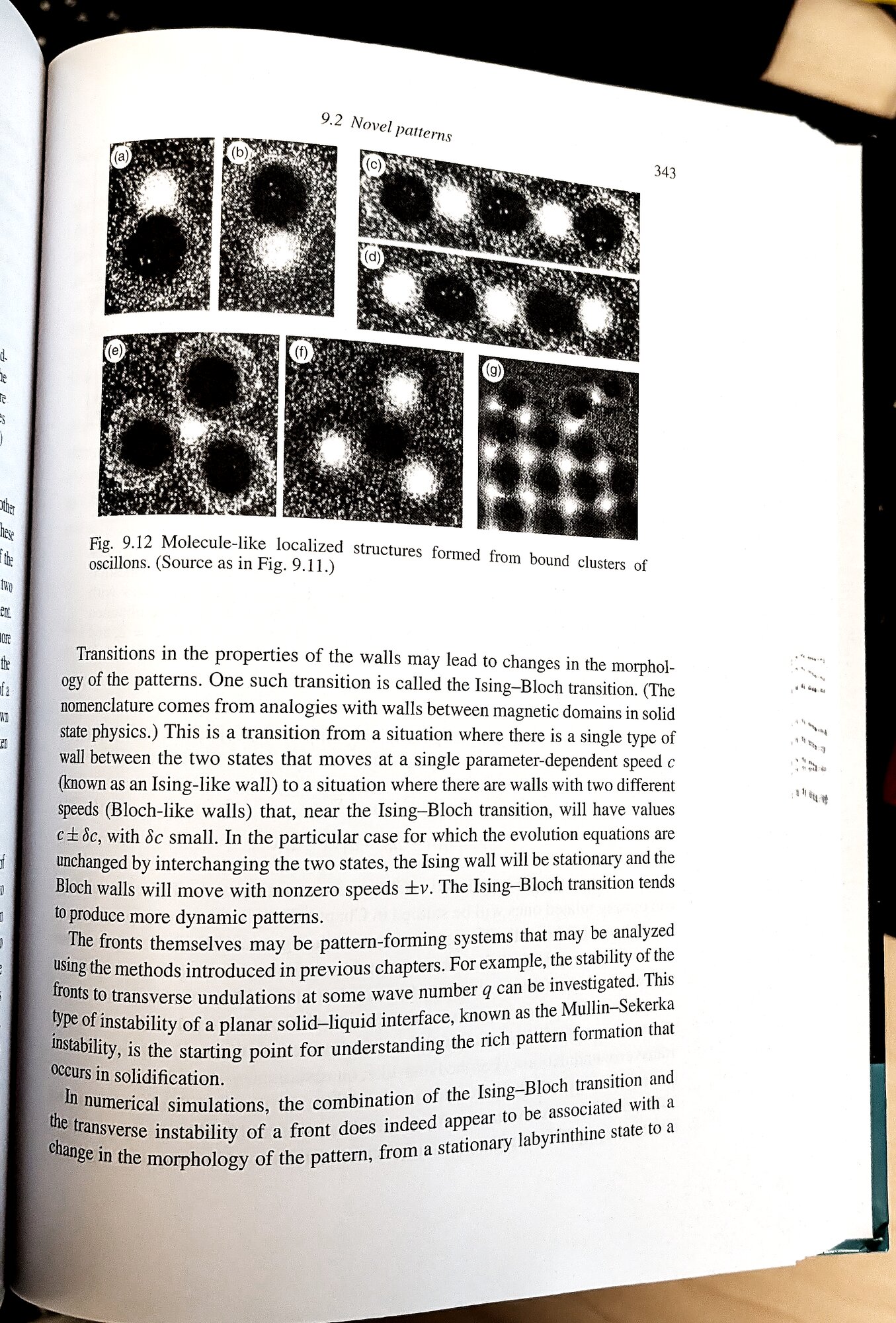
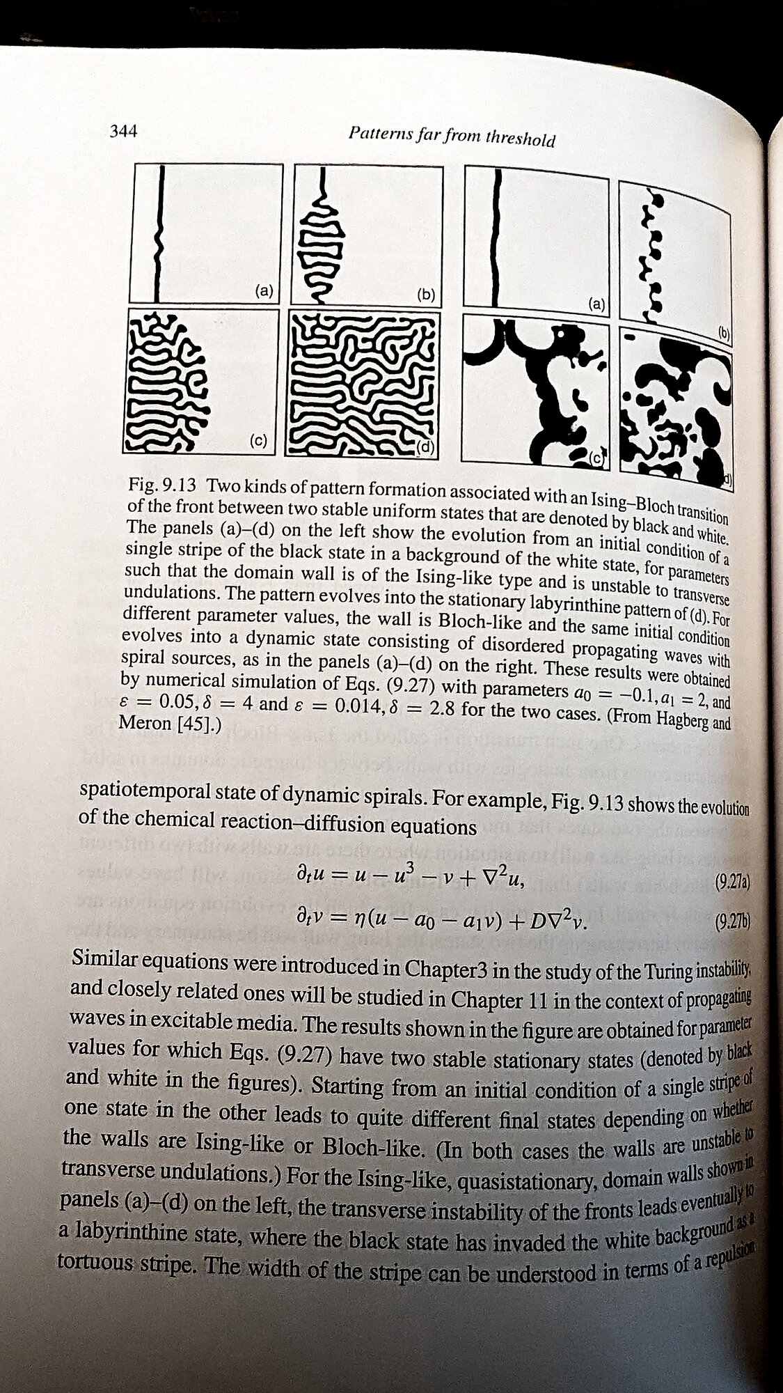
The ice-neuron morphology suddenly had the right language. A moving interface, driven by a transported field, can become morphologically unstable. The branching did not need a neural explanation because there was already a beautiful piece of nonequilibrium physics that told me how the silhouette could arise.
And once that was clear, the rest of the problem could be posed properly.
Instead of asking, Why does ice look like a neuron?, I could ask:
What has to be added to the physics of the ice before the dendritic silhouette becomes a dynamical motif?
That is a much better question.
The rest was a matter of going step by step: branching and branching, like the ice neurons themselves, but now with purpose and with a map. Growth instability. Internal state. Field source. Feedback. Freeze the geometry. Ask what remains.
Very much the way Claude had taught me to move through a problem: follow the physics through the equations and do not jump ahead of what the system actually possesses.
The silhouette fallacy
Walden gave me a useful inversion.
The ice neuron was not interesting because ice had somehow discovered neuroscience. It was interesting because it had acquired the thing most likely to fool us — the shape — while withholding almost everything else we normally smuggle into the word neuron.
A dendritic silhouette is so strongly associated with a neuron that it is tempting to let the picture do the reasoning for us. Branching becomes computation. A motif in the geometry becomes a motif in the dynamics. A tree that looks neuronal quietly inherits the properties of a neuron.
I call that the silhouette fallacy.
The paper is an attempt to make that mistake mathematically difficult to commit.
Ice is not pretending to be a neuron
The resemblance between ice and dendrites is not mysterious. It is not even especially biological.
A front advancing through a transported field can become unstable. Small perturbations grow, tips compete for flux, curvature suppresses very small features, and a branching structure emerges. Crystal growth does this. Diffusion-limited aggregation does this. Many biological growth processes do this. Neuronal arbors can share some of the same geometric statistics because the physics of making a cheap branching tree is not unique to neurons.
So the first lesson is almost disappointingly simple:
A branching form can be evidence of a growth instability without being evidence of a computation.
This matters because the word motif is often asked to do two different jobs.
One meaning is structural: a recurring or overrepresented piece of a graph.
The other is dynamical: a primitive that does something when driven — filters, persists, oscillates, selects, amplifies.
Ice can have the first kind of motif. It can grow the same little branching shapes over and over.
That does not give it the second.
A silhouette is morphology. A dynamical motif needs a state.
The missing state
This is the first real separation in the paper.
Imagine freezing the geometry of a dendrite. The tree no longer grows. But if it is a biological dendrite, the object is not dead mathematically just because its shape is fixed. Membrane voltage still evolves. Channels still open and close. Local nonlinearities remain. Excitable events can propagate.
That is already something ice does not possess.
So I add an internal state to the interface. I use a minimal excitable system because the point is not to reproduce a membrane channel by channel. The point is to give the interface degrees of freedom that can evolve on their own, even after the geometry is frozen.
At that point we have moved from an ice neuron to an active cable.
But that is still not the full distinction I wanted.
A biological neuron does not merely carry dynamics along its own cable.
It also changes the field around it.
The neuron is not only in the field. It writes the field.
This is where ephaptic coupling enters the story.
Neural activity generates extracellular electric fields. Those fields are not just pretty measurements sitting outside the “real” computation. They are produced by membrane currents, and they can in turn act back on excitable membranes.
So there is a physical loop:
membrane state → extracellular field → membrane state
The neuron is therefore not only a consumer of its environment. It is one of the authors of the environment that subsequently acts on it.
That is the step I call field closure.
In the model, almost the entire conceptual distinction is carried by one parameter, $\gamma$.
When
\[\gamma = 0,\]the interface responds to the field but does not contribute an independent state-dependent source back into it.
That is the ice limit.
When
\[\gamma > 0,\]the internal state writes into the field, and the field feeds back onto subsequent dynamics.
The object has closed a physical loop.
The point of $\gamma$ is not that neurons have a literal knob called gamma. The point is that it lets the same mathematical object cross a very clean conceptual boundary:
passive silhouette → field-closed dynamical system.
Why closure, rather than just feedback?
Because feedback is cheap too.
Many physical systems feed back on themselves. That alone does not make them computers.
I use closure here in a deliberately restricted sense. Field closure means that an internally realized physical state contributes to a field and that this field then changes the future dynamics of the state.
That is already stronger than a structure merely responding to an imposed environment.
But it is still weaker than what I have elsewhere called computational closure.
The distinction matters.
In physical computing, one should not be able to declare an arbitrary physical trajectory a computation simply by inventing a convenient encoding afterward. The computational description has to correspond to the physical organization of the system.
And in the stronger autonomous case, internally realized readout states must participate in selecting what happens next.
Field closure does not automatically guarantee that.
It supplies the physical loop.
Whether the loop realizes a computation in the stronger sense depends on the transition structure, the readout, and what operations the dynamics actually implement.
So I think of the hierarchy this way:
- structure gives the object a shape;
- internal state gives it autonomous dynamics;
- field closure lets those dynamics modify the medium that acts back on them;
- computational closure, when present, is a further claim about what that closed physical loop implements.
The distinctions are easy to blur because all four can live in the same biological object.
The ice neuron separates them for us.
One knob deforms the physics
Once the loop is switched on, it does not merely add a decorative correction.
The field-coupled state changes the growth spectrum of the interface. In the ice limit, the familiar morphological instability selects the growing modes. With finite closure, those modes are shifted and amplified.
More interestingly, the coupled system can become oscillatory in a region where the isolated internal oscillator is still quiescent.
That is important conceptually.
The oscillation is not simply “the neuron already oscillated and then we attached it to a tree.” The coupling itself opens a dynamical region unavailable to the isolated state.
The field is therefore not just carrying activity from one place to another.
It changes what dynamics are available to the combined system.
This is one reason I find the physics of ephaptic coupling more interesting than treating it as a small correction to ordinary cable theory. Even a weak shared field can alter the effective dynamical object because it changes the closure of the system.
Freeze the tree
But a spectrum on a growing interface still leaves an obvious objection.
Perhaps all we have done is change the growth.
Perhaps the field-closed system looks different because it grows differently.
So the cleanest test is to remove growth entirely.
Grow the tree with (\gamma=0).
Freeze its geometry.
Then turn on finite (\gamma).
Now the morphology cannot save the argument. The branches are identical before and after. The graph is identical. The cable is identical.
Only the closure changes.
In the assay, two distant tips are driven and another distant tip is read out. At (\gamma=0), transmission has to work through the active cable. At finite (\gamma), the state-generated field adds spatial interactions that do not follow the cable graph.
Persistence at the readout increases.
That sentence is the heart of the paper:
The shape no longer changes; only the dynamical closure does.
So the extra effect cannot be credited to the silhouette.
And because the first-order contribution can be decomposed spatially, one can ask where the closure actually does its work.
The answer is not “everywhere in the dendritic shape.”
A small set of field-mediated shortcuts contributes most strongly.
The dynamical motif is therefore not the outline of the tree. It is a set of physical interactions that the outline does not contain.
That is a much more demanding use of the word motif.
The graph is not the whole architecture
This is where the ephaptic story becomes especially relevant to neuroscience.
A cable graph gives one geometry of interaction: current flows along the neurite.
A synaptic connectome gives another: activity moves through synaptic edges.
But an extracellular field introduces a different geometry altogether. It depends on space, conductivity, screening, tissue organization, and the activity of the surrounding population.
Two compartments that are far apart along the cable can be close through the field.
So the physical interaction graph need not be the anatomical graph.
This is not a semantic detail.
If computation is implemented by the physical degrees of freedom of the nervous system, then the effective architecture is whatever set of interactions those degrees of freedom actually realize.
The extracellular field is part of that substrate.
It does not have to dominate every regime to matter conceptually. Its existence already tells us that the neuron is not exhausted by a tree of compartments connected only by cable edges.
The system can write nonlocal couplings into the medium around itself.
Three possessions
The whole paper can be compressed into three rows:
| object | growth structure | internal dynamics | field feedback |
|---|---|---|---|
| ice neuron | ✓ | – | – |
| active cable | ✓ | ✓ | – |
| field-closed neuron | ✓ | ✓ | ✓ |
I like this hierarchy because each row possesses something the previous one does not.
The ice neuron has the branching structure.
The active cable adds an internal state.
The field-closed neuron adds the loop by which that state writes into a shared physical field and receives the consequences back.
A silhouette census cannot distinguish these rows.
That is exactly why the silhouette is dangerous.
The physical-computing lesson
The broader point is not really about ice.
It is about what we mean when we say that a physical object computes.
There is a strong temptation to identify computation with form: a network, a circuit diagram, a dendritic tree, a lattice, a reservoir.
But the physical computation is not in the picture.
It is in the organized evolution of physical states.
A useful architecture has to specify not only where the degrees of freedom sit, but what states they possess, how those states transform, and what parts of the physical substrate those transformations can modify.
Field closure is one concrete mechanism by which the substrate becomes an active participant rather than a passive stage.
The membrane writes the field.
The field rewrites the conditions for the membrane.
The “wiring” is therefore partly produced dynamically by the physics itself.
That is much closer to the kind of object I want to call a physical computer.
And the NeuroAI lesson
This is also why I am cautious about biomimetic geometry in NeuroAI.
A dendrite-inspired architecture can be useful.
A branched neuromorphic device can be useful.
A network can borrow the visual language of a neuron and still do something interesting.
But resemblance is not inheritance.
If all we copied is the tree, then in the hierarchy above we have copied the first row.
We have copied the ice neuron.
To move beyond that, the branches need internal dynamical states.
And to recover the field-closed organization, those states must be able to write into some shared physical variable that acts back on the computation.
It does not have to be an extracellular electric field. It could be optical, mechanical, chemical, acoustic, electromagnetic, or some other collective physical mode.
The essential feature is not the material.
It is the loop:
state writes field; field acts on state.
That is the structural motif I care about.
Not the silhouette.
The fallacy, in one sentence
Pond ice can look like a neuron because a growth instability is enough to draw the tree.
A biological neuron is different because the tree carries an internal state, and that state can help write the field that acts back on the tree.
That is the contrast.
Shape is morphology without an internal state and a source term. That is the ice neuron.
Excitability adds an active cable.
Field closure is the biophysical mélange in which the neuron writes part of the field that then acts back on it. That is the biological neuron.
The pond can draw the silhouette.
It cannot close the loop.
I hope Papa Prigogine would be proud.
And then there are the patterns that refuse even my best attempt at a story.
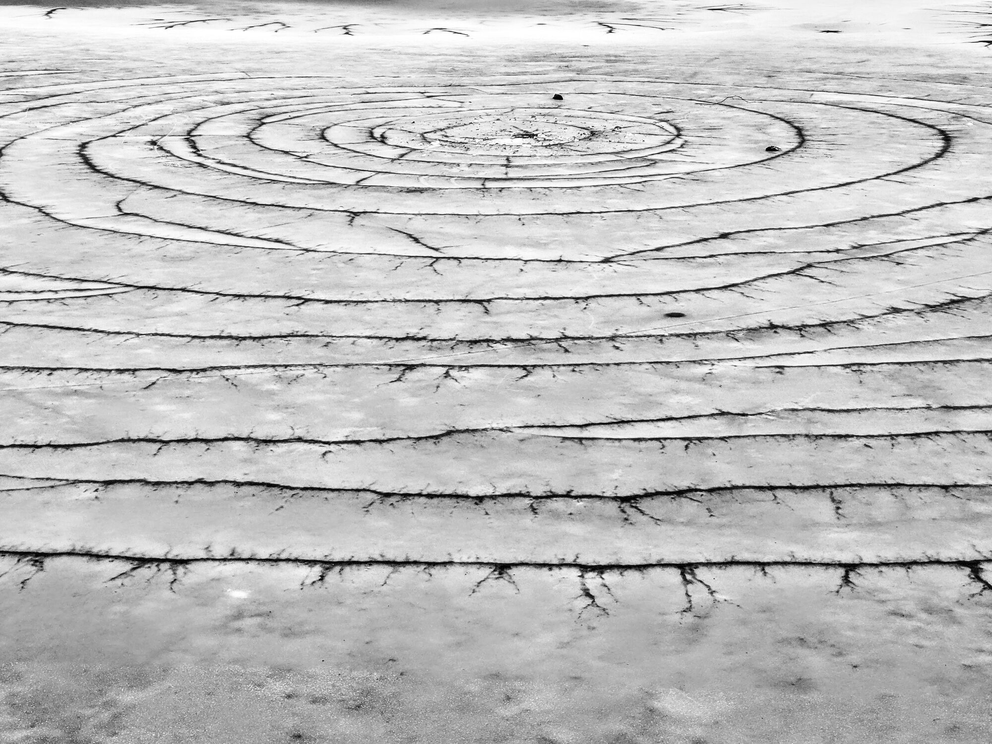
Here is one pattern that I have no explanation for. And no, it is not from Mars! It is the same place, Walden pond, same day. If you have a hunch, you know who to call.
Cite this post
@misc{dehghani2026SilhouetteFallacy,
  author       = {Nima Dehghani},
  title        = {{The Silhouette Fallacy}},
  year         = {2026},
  howpublished = {\url{https://neurovium.science/posts/pblog-IceNeuron/}},
  note         = {Companion post to: Field closure, ice neurons, and when a dendrite is a motif
                  (2026). doi:10.48550/arXiv.2610.00184}
}